
Skeletonizing an Image in 3D
Brett's Pick this week is Skeleton3D, by Philip Kollmansberger.
A couple years ago, I put together a demo to show how to use MATLAB to calculate the tortuosity, or “twistedness,” of blood vessels. There are different formulas for measuring that property, but perhaps the easiest way of determining tortuosity of a path is using the arc-chord ratio—i.e., the length of the curve divided by the distance between its endpoints.
In my demo, I assumed the vessels were 2-dimensional, and then used some Image Processing Toolbox functionality to: 1) skeletonize the vessels of interest using bwmorph/skel, and 2) determine the endpoints of the segment (facilitated by a call to bwmorph/endpoints. Then, using one or both endpoints of the segment, respectively, to 3) calculate the geodesic distance transform of the vessel (bwdistgeodesic), the maximum value of which provides the arc-length; and 4) calculate the distance the endpoints. (You can find a discussion of this approach in a recorded webinar at mathworks.com.)
This approach is reasonably straightforward when you assume planarity, but in 3D, it gets much more challenging—because bwmorph doesn’t currently support the analysis of 3D images. That leaves us struggling to do the skeletonization- and endpoint-detection steps.
Enter Philip’s Skeleton3D function. Using an algorithm (properly cited in the code) based on “3-D medial surface/axis thinning algorithms,” Skeleton3D finds axial values that can be subsequently analyzed for the determination of tortuosity.
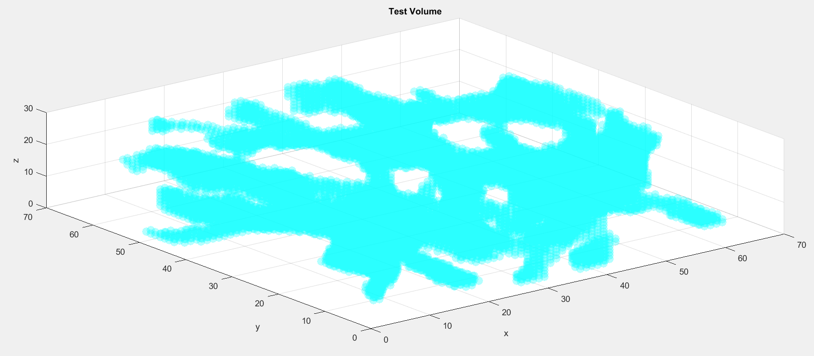
load testvol
inds = find(testvol);
[y,x,z] = ind2sub(size(testvol),inds);
s = scatter3(x,y,z,100,...
  'Marker','o',...
  'MarkerEdgeColor','none',...
  'MarkerFaceAlpha',0.3,...
  'MarkerFaceColor','c');
xlabel('x');
ylabel('y');
zlabel('z');
title('Test Volume')
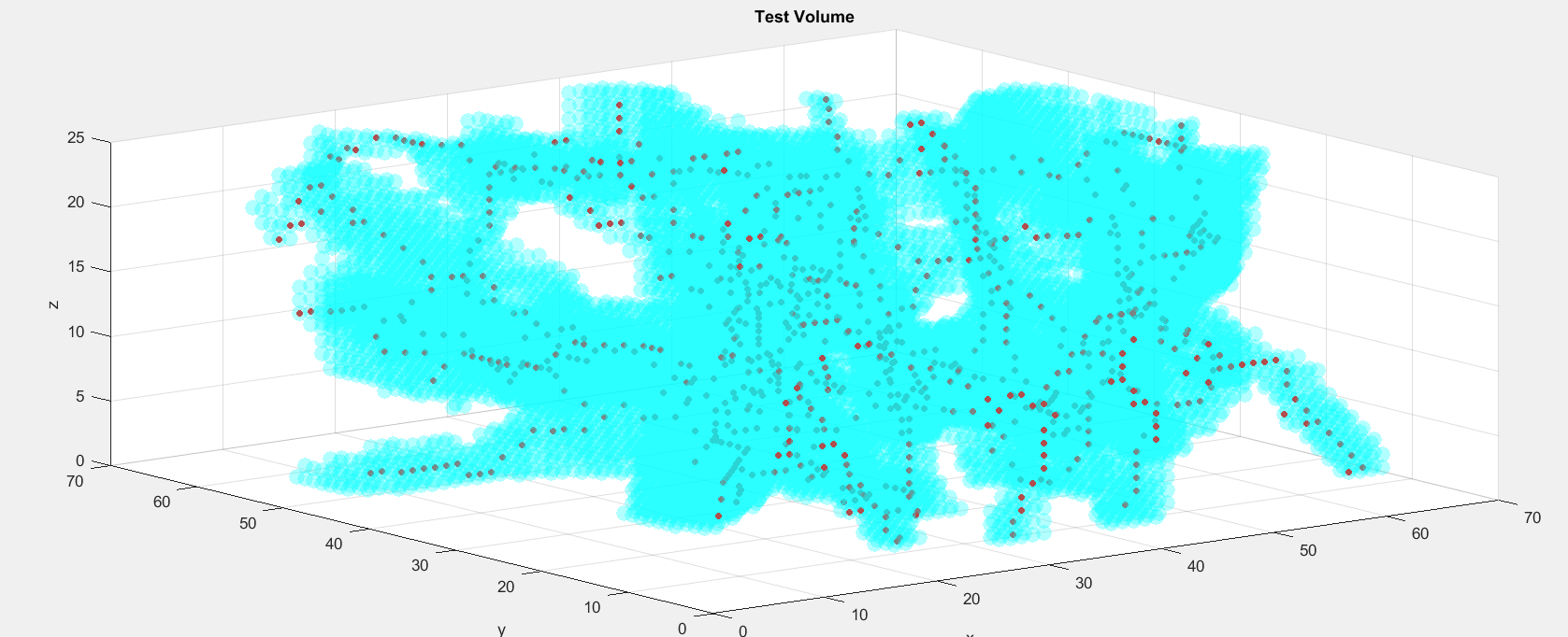
Now we can extract and display points along the skeleton of this test volume:
skel = Skeleton3D(testvol);
inds = find(skel);
[yskel,xskel,zskel] = ind2sub(size(skel),inds);
hold on
p2 = scatter3(xskel,yskel,zskel,20,...
    'Marker','o',...
    'MarkerEdgeColor','none',...
    'MarkerFaceColor','r');
For tortuosity determinations, there's still some more work to be done--we still need to detect endpoints and arclengths, for instance. Those are topics for a different day.
For Philip, an implementation comment: Skeleton3D is considerably slower than it needs to be. It relies on looping over indices where vectorized approaches can be much faster. And converting to logical indexing for comparisons can also speed things up. For instance:
In the determination of "candidate foreground voxels," you can replace:
cands = intersect(find(cands(:)==1),find(skel(:)==1));
with
cands = find(cands & skel);
(Admittedly, that buys just a little improvement in performance, but I find it more elegant.)
More pointedly, if you were to profile your code, you'd find a large percentage of time spent calculating the skeleton of your testvol reflects nearly 87,000 calls to p_oct_label. That code could be greatly sped up by replacing successive indx(row) = find(cube(row,:)==1) calls in the analysis of 'cube' with something along the lines of
[row,col] = ind2sub(size(cube),cube==1);
indx(row) = col(row == 1);
and iterating over values of row.
Nonetheless, this provides a good start to anyone needing to skeletonize structures in 3D. Thanks, Philip, for this very nice contribution!
As always, I welcome your thoughts and comments.
- カテゴリ:
- Picks


コメント
コメントを残すには、ここ をクリックして MathWorks アカウントにサインインするか新しい MathWorks アカウントを作成します。