Tetrahedral interpolation for colorspace conversion
The Image Processing Toolbox function applycform can convert colors based on ICC profiles. ICC standards for the International Color Consortium, and an ICC profile typically contains information about the color characteristics of a particular device. Specifically, the profile contains data used to transform colors between the device-specific colorspace and the device-independent colorspaces L*a*b* or XYZ. These colorspace transformations can be quite complicated, and a profile may contain parametric curves, matrix multiplications, one-dimensional lookup tables, and multidimensional lookup tables. Many contain all of the above.
applycform today uses trilinear interpolation for profiles containing three-dimensional lookup tables (or quadrilinear for four-dimensional tables). Some of our color science customers have been recommending that we switch to something called tetrahedral interpolation instead.
In both tetrahedral and trilinear interpolation the grid points along each of the three axes serve to divide the volume into a set of rectangular hexahedra. To interpolate at a particular point, the first step is determine which hexahedron the point is in. In tetrahedral interpolation, the hexahedron is further subdivided into six tetrahedra. There is more than one possible subdivision. Here's the subdivision typically used for colorspace conversion applications.
% Form the eight vertices of a cube.
vertices = [0 0 0
    1 0 0
    0 0 1
    1 0 1
    0 1 0
    1 1 0
    0 1 1
    1 1 1];
One of the tetrahedra contains 1st, 2nd, 6th, and 8th vertices. The function nchoosek gives us a convenient way to compute the corresponding faces.
f = nchoosek([1 2 6 8], 3)
f =

     1     2     6
     1     2     8
     1     6     8
     2     6     8
Here are the faces for all six of the tetrahedra.
faces{1} = nchoosek([1 2 6 8], 3);
faces{2} = nchoosek([1 5 6 8], 3);
faces{3} = nchoosek([1 3 7 8], 3);
faces{4} = nchoosek([1 5 7 8], 3);
faces{5} = nchoosek([1 3 4 8], 3);
faces{6} = nchoosek([1 2 4 8], 3);

colors = jet(numel(faces));

ec = 'black';
fa = 0.2;

close all
for k = 1:numel(faces)
    tetra{k} = patch('Vertices', vertices, 'Faces', faces{k}, ...
    'FaceColor', colors(k,:), 'EdgeColor', ec, 'FaceAlpha', fa);
end

view(3)
axis equal
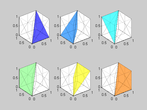
That's a little hard to see, so let's show the individual tetrahedra in separate plots.
fa = 0.4;
ea = 0.1;
for k = 1:6
    subplot(2,3,k)
    for p = 1:6
            tetra{p} = patch('Vertices', vertices, 'Faces', faces{p}, ...
              'FaceColor', 'none', 'EdgeColor', ec, 'EdgeAlpha', ea);
    end
    set(tetra{k}, 'FaceColor', colors(k,:), 'FaceAlpha', fa);
    axis equal
    axis([0 1 0 1 0 1])
    view(3)
    grid on
end

Once the tetrahedron containing the interpolation point is identified, the interpolation is computed as a weighted sum of the grid values at the vertices of that tetrahedron.
If you look carefully at each of the tetrahedra, you can see that each one shares a common edge that is the diagonal from (0,0,0) to (1,1,1). That's why this particular tetrahedral subdivision is typically used for colorspace conversions. In an RGB space, this diagonal contains the neutral (or gray) colors, which are particularly important. Tetrahedral interpolation can be used to convert colors more accurately and with lower computational cost.
We now have a patch available online that updates applycform to use tetrahedral interpolation. If color science is your game and you use the ICC-related functions in the toolbox, then I invite you to download and try the patch.
If you want to know more about interpolation methods used for colorspace conversions, you might find this paper to be useful:
Kasson, Nin, Plouffe, and Hafner, "Performing color space conversions with three-dimensional linear interpolation," Journal of Electronic Imaging, July 1995, Vol. 4(3), pp. 226-250.
 Cleve’s Corner: Cleve Moler on Mathematics and Computing
 The MATLAB Blog
 Guy on Simulink
 MATLAB Community
 Artificial Intelligence
 Developer Zone
 Stuart’s MATLAB Videos
 Behind the Headlines
 File Exchange Pick of the Week
 Hans on IoT
 Student Lounge
 MATLAB ユーザーコミュニティー
 Startups, Accelerators, & Entrepreneurs
 Autonomous Systems
 Quantitative Finance
 MATLAB Graphics and App Building


评论
要发表评论,请点击 此处 登录到您的 MathWorks 帐户或创建一个新帐户。