Filtering fun

Posted by Steve Eddins, July 22, 2011

5 views (last 30 days) | 0 Likes | 4 comments

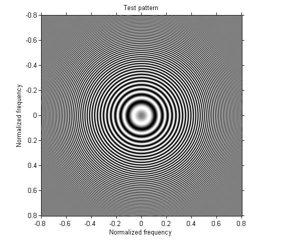
Today I want to take the test pattern I created last time and subject it to a variety of frequency-based filters.

In this post I'll be using a variety of frequency design and frequency-response visualization tools in MATLAB, Signal Processing Toolbox, and Image Processing Toolbox, including fir1, ftrans2, freqspace, fwind1, and freqz2. I won't be giving much explanation of these filter design techniques. Perhaps in the future I'll explore filter design here in more detail. For now, though, I really just want to have some fun with this test pattern.

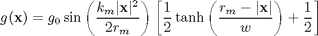
[x,y] = meshgrid(-200:200);
r = hypot(x,y);
km = 0.8*pi;
rm = 200;
w = rm/10;
term1 = sin( (km * r.^2) / (2 * rm) );
term2 = 0.5*tanh((rm - r)/w) + 0.5;
g = (term1 .* term2 + 1) / 2;

imshow(g, 'XData', [-.8 .8], 'YData', [-.8 .8])
axis on
xlabel('Normalized frequency'), ylabel('Normalized frequency')
title('Test pattern')

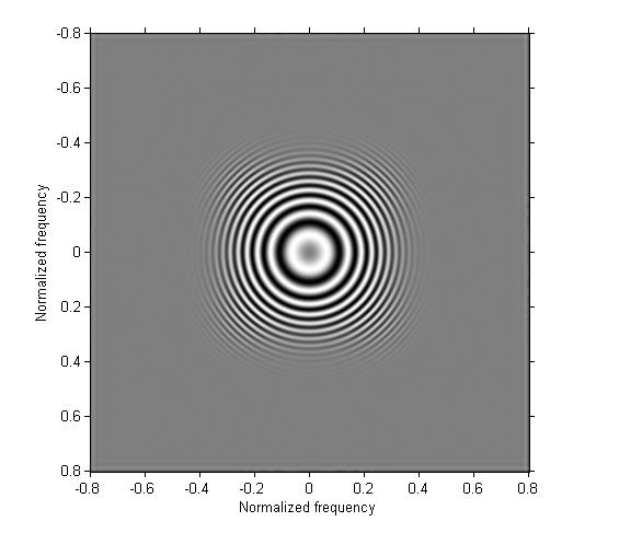
Example 1: Design a one-dimensional lowpass filter and apply it in both directions.

b = fir1(30,0.3);
h = b' * b;
g1 = imfilter(g, h);

imshow(g1, 'XData', [-.8 .8], 'YData', [-.8 .8])
axis on
xlabel('Normalized frequency'), ylabel('Normalized frequency')

Example 2: Design a one-dimensional highpass filter and apply it in both directions.

b2 = fir1(30, 0.3, 'high');
h2 = b2' * b2;
g2 = imfilter(g, h2);

imshow(g2, [], 'XData', [-.8 .8], 'YData', [-.8 .8])
axis on
xlabel('Normalized frequency'), ylabel('Normalized frequency')

Example 3: Design a one-dimensional bandpass filter and apply it on both directions.

b3 = fir1(30, [0.3 0.4]);
h3 = b3' * b3;
g3 = imfilter(g, h3);

imshow(g3, [], 'XData', [-.8 .8], 'YData', [-.8 .8])
axis on
xlabel('Normalized frequency'), ylabel('Normalized frequency')

Example 4: Apply the one-dimensional bandpass filter from the previous step in only one direction.

g4 = imfilter(g, b3);

imshow(g4, [], 'XData', [-.8 .8], 'YData', [-.8 .8])
axis on
xlabel('Normalized frequency'), ylabel('Normalized frequency')

Example 5: Use ftrans2 to turn the one-dimensional bandpass filter from the previous example into a two-dimensional bandpass filter that is approximately circularly symmetric.

h5 = ftrans2(b3);
g5 = imfilter(g, h5);

imshow(g5, [], 'XData', [-.8 .8], 'YData', [-.8 .8])
axis on
xlabel('Normalized frequency'), ylabel('Normalized frequency')

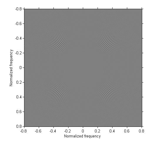
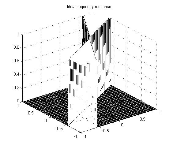
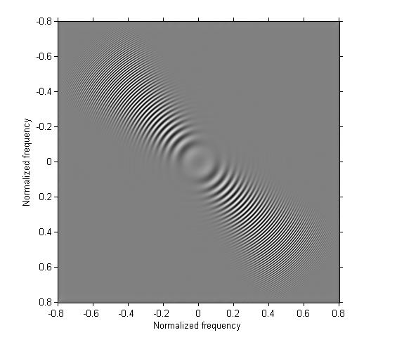
Example 6: Use fwind1 to design a two-dimensional filter that has a wedge-shaped frequency response.

[f1, f2] = freqspace(101, 'meshgrid');
theta = cart2pol(f1, f2);
Hd = ((theta >= pi/6) & (theta < pi/3)) | ...
    ((theta >= -5*pi/6) & (theta < -2*pi/3));
mesh(f1, f2, double(Hd))
title('Ideal frequency response')

h6 = fwind1(Hd, hamming(31));
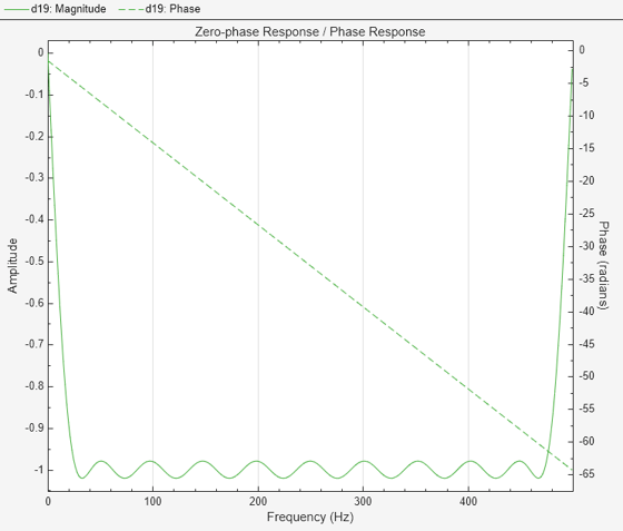
freqz2(h6)
title('Designed filter frequency response')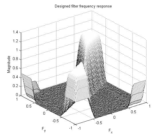

g6 = imfilter(g, h6);

imshow(g6, [], 'XData', [-.8 .8], 'YData', [-.8 .8])
axis on
xlabel('Normalized frequency'), ylabel('Normalized frequency')

Example 7: Compare the use of an averaging filter and a Gaussian filter. This example is inspired by Cris Luengo's comment from last week.

g7 = imfilter(g, fspecial('average', 9));
imshow(g7, [], 'XData', [-.8 .8], 'YData', [-.8 .8])
axis on
xlabel('Normalized frequency'), ylabel('Normalized frequency')
title('13-by-13 averaging filter')

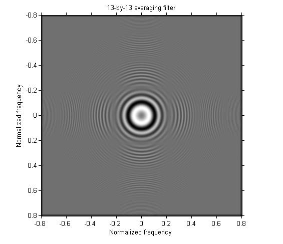
You can see that some very high frequencies remain in the output. The Gaussian filter performs much better:

g9 = imfilter(g, fspecial('gaussian', 9, 2));
imshow(g9, [], 'XData', [-.8 .8], 'YData', [-.8 .8])
axis on
xlabel('Normalized frequency'), ylabel('Normalized frequency')
title('13-by-13 Gaussian filter')