I'd like to welcome back my fellow MATLAB Central blogger Brett Shoelson for the last in a three-part series on extracting curve values from a plot. You can find Brett over at the File Exchange Pick of the Week blog, or you can check out his many File Exchange contributions. -Steve

Contents

Quick recap

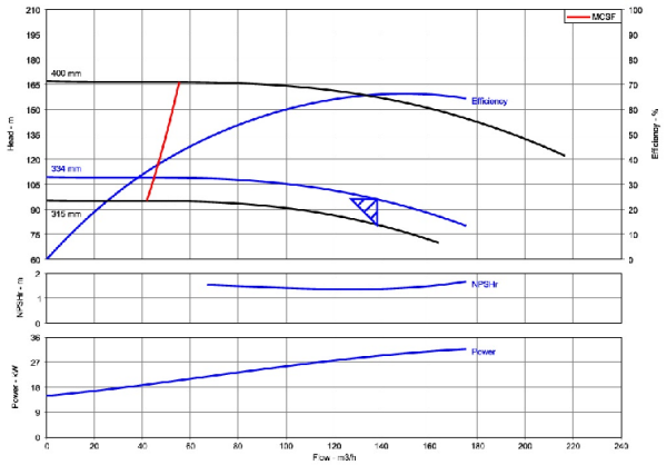
If you've followed Steve's blog for the past couple weeks, you'll know that Steve has graciously allowed me to demonstrate how one might extract real data from a graphical depiction of the data. In this final post in this three-part series, I will use the coordinates I extracted from the curve of interest to fit a predictive model to those data. Recall that I showed two approaches to determine the x- y- coordinates of the efficiency curve:

First, load the variables xs, ys, and bb, which were computed in the previous post.

tempfile = [tempname '.mat'];
url = 'https://blogs.mathworks.com/images/steve/2013/curve.mat';
urlwrite(url,tempfile);
s = load(tempfile);
xs = s.xs;
ys = s.ys;
bb = s.bb;
delete(tempfile);

Clearly, the results obtained using regionprops were better than those I got using bwtraceboundary. We may as well use those values for our curve fit. Before we do that, though, it will be useful to transform the data to account for the fact that the extracted coordinates are in units of pixels, rather than units of flow rate and efficiency. I do that manually here:

flowLims = [0 240];
efficiencyLims = [0 100];

% Scale data to specified limits for curvefit
% Scale xs:
xs  = (xs-bb(1))/bb(3)*diff(flowLims)+flowLims(1);
% Scale ys:
ys = (bb(2)+bb(4)-ys)/bb(4); %Percentages = Efficiencies

(By the way, if you ever need to fit data to anything other than a very simple polynomial, and if you don't have the Curve Fitting Toolbox, I hope this motivates you to get it; it is is an excellent tool that will make your life much easier!)

You can fit to just about any type of equation that makes sense. (You can even provide a custom equation, if you have one in mind.) I can, for instance, get a reasonably good robust "Bisquare" fit using a two-term exponential. Or, since I just want to represent my data, and not force them to a specific form, I could fit them to a smoothing spline.

cftool(xs,ys)

When you've interactively selected your fit options, you can readily tell MATLAB to generate code, with which you can apply the same routine to subsequent images (data sets).

Here's the code that cftool told me to use:

[xData, yData] = prepareCurveData( xs, ys );

% Set up fittype and options.
ft = fittype( 'smoothingspline' );
opts = fitoptions( 'Method', 'SmoothingSpline' );
opts.SmoothingParam = 0.004;

% Fit model to data.
[fitresult, gof] = fit( xData, yData, ft, opts );

% Plot fit with data.
figure( 'Name', 'untitled fit 1' );
h = plot( fitresult, xData, yData );
legend( h, 'ys vs. xs', 'untitled fit 1', 'Location', 'NorthEast' );
% Label axes
xlabel( 'xs' );
ylabel( 'ys' );
grid on

We could, for illustration, calculate the efficiency of the pump when the flow rate is 100 m^3/hr:

flow100 = fitresult(100)

flow100 =

    0.5997

If you refer to the original image, you'll see that that value perfectly reflects the efficiency at the specified flow rate!

Final comment

I don't really have a good sense for how well this exact approach will work for subsequent images. I tried to make the code fairly general, but the automatability of the problem depends markedly on the ability to exploit similarities in the data set (images). Therein lies the art of image processing!

The complete series

Get the MATLAB code

Published with MATLAB® R2013b

Published with MATLAB® R2013b