Image binarization – Otsu’s method
In my 16-May-2016 post about image binarization, I talked about the new binarization functions in R2016a. Today I want to switch gears and talk about Otsu's method, one of the algorithms underlying imbinarize.
(A bonus feature of today's blog post is a demo of yyaxis, a new feature of MATLAB R2016a.)
Otsu's method is named for Nobuyuki Otsu, who published it in IEEE Transactions on Systems, Man, and Cybernetics, vol. SMC-9, no. 1, January 1979. At this time, researchers had already explored a variety of ways to choose a threshold automatically by examining the histogram of image pixel values. The basic idea is to look for two peaks, representing foreground and background pixel values, and pick a point in between the two peaks as the threshold value.
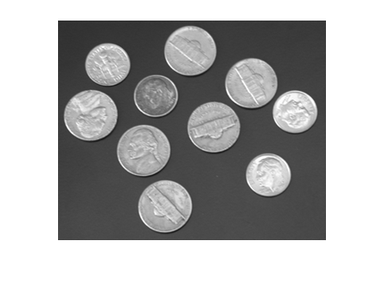
Here's a simple example using the coins image.
I = imread('coins.png');
imshow(I)
imhist(I)
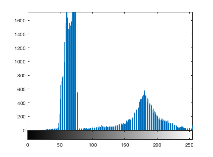
The function imbinarize calls otsuthresh to get a normalized threshold value.
t = otsuthresh(histcounts(I,-0.5:255.5))
t =

    0.4941
Let's see where that threshold is.
hold on
plot(255*[t t], ylim, 'r', 'LineWidth', 5)
hold off
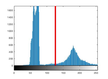
And here is the thresholded coins image.
imshow(imbinarize(I,t))

How does this threshold selection work? It is based on entirely on the set of histogram counts. To show the computation, I'll adopt the notation from the paper. Pixels can take on the set of values $i = 1,2,\ldots,L$. The histogram count for pixel value $i$ is $n_i$, and the associated probability is $p_i = n_i/N$, where $N$ is the number of image pixels. (I'm using the word probability here somewhat loosely, in the relative frequency sense.)
The thresholding task is formulated as the problem of dividing image pixels into two classes. $C_0$ is the set of pixels with values $[1,\ldots,k]$, and $C_1$ is the set of pixels with values in the range $[k+1,\ldots,L]$.
The overall class probabilities, $\omega_0$ and $\omega_1$, are:
$$\omega_0 = \sum_{i=1}^k p_i = \omega(k)$$
$$\omega_1 = \sum_{i=k+1}^L p_i = 1 - \omega_0(k)$$
The class means, $\mu_0$ and $\mu_1$, are the mean values of the pixels in $C_0$ and $C_1$. They are given by:
$$\mu_0 = \sum_{i=1}^k i p_i / \omega_0 = \mu(k)/\omega(k)$$
$$\mu_1 = \sum_{i=k+1}^L i p_i / \omega_1 = \frac{\mu_T - \mu(k)}{1 - \omega(k)}$$
where
$$\mu(k) = \sum_{i-1}^k i p_i$$
and $\mu_T$, the mean pixel value for the total image, is:
$$\mu_T = \sum_{i=1}^L i p_i.$$
The class variances, $\sigma_0^2$ and $\sigma_1^2$, are:
$$\sigma_0^2 = \sum_{i = 1}^k (i - \mu_0)^2 p_i / \omega_0$$
$$\sigma_1^2 = \sum_{i = k+1}^L (i - \mu_1)^2 pi / \omega_1.$$
Otsu mentions three measures of "good" class separability: within-class variance ($\lambda$), between-class variance ($\kappa$), and total variance ($\eta$). These are given by:
$$\lambda = \sigma_B^2$$
$$\kappa = \sigma_T^2/\sigma_W^2$$
$$\eta = \sigma_B^2/\sigma_T^2$$
where
$$\sigma_W^2 = \omega_0 \sigma_0^2 + \omega_1 \sigma_1^2$$
$$\sigma_B^2 = \omega_0 (\mu_0 - \mu_T)^2 + \omega_1 (\mu_1 - \mu_T)^2 = \omega_0 \omega_1 (\mu_1 - \mu_0)^2.$$
He goes on to point out that maximizing any of these criteria is equivalent to maximizing the others. Further, maximizing $\eta$ is the same as maximizing $\sigma_B^2$, which can be rewritten in terms of the selected threshold, $k$:
$$ \sigma_B^2(k) = \frac{[\mu_T \omega(k) - \mu(k)]^2}{\omega(k) [1 - \omega(k)]}.$$
The equation above is the heart of the algorithm. $\sigma_B^2$ is computed for all possible threshold values, and we choose as our threshold the value that maximizes it.
OK, that was a lot of equations, but there's really not that much involved in computing the key quantity, $\sigma_B^2(k)$. Here's what the computation looks like for the coins image.
counts = imhist(I);
L = length(counts);
p = counts / sum(counts);
omega = cumsum(p);
mu = cumsum(p .* (1:L)');
mu_t = mu(end);

sigma_b_squared = (mu_t * omega - mu).^2 ./ (omega .* (1 - omega));
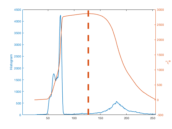
Using yyaxis, a new R2016a feature, let's plot the histogram and $\sigma_B^2$ together.
close all
yyaxis left
plot(counts)
ylabel('Histogram')

yyaxis right
plot(sigma_b_squared)
ylabel('\sigma_B^2')

xlim([1 256])
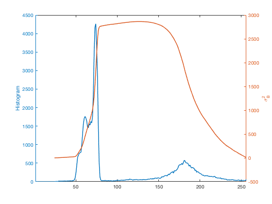
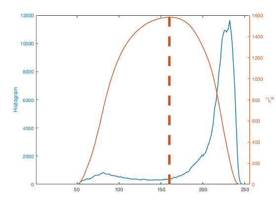
Otsu's method chooses the place where $\sigma_B^2$ is the highest as the threshold.
[~,k] = max(sigma_b_squared);
hold on
plot([k k],ylim,'LineWidth',5)
hold off
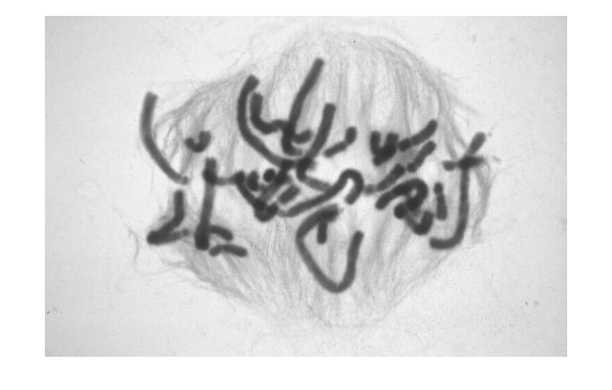
Here's another example. This is a public-domain light microscope image of Lily mitosis. (The original image is courtesy Andrew S. Bajer, University of Oregon, Eugene, OR. This version is slightly cropped.)
url = 'https://blogs.mathworks.com/steve/files/205.jpg';
I = rgb2gray(imread(url));
clf
imshow(I)
counts = imhist(I);
L = length(counts);
p = counts / sum(counts);
omega = cumsum(p);
mu = cumsum(p .* (1:L)');
mu_t = mu(end);

sigma_b_squared = (mu_t * omega - mu).^2 ./ (omega .* (1 - omega));

close all
yyaxis left
plot(counts)
ylabel('Histogram')

yyaxis right
plot(sigma_b_squared)
ylabel('\sigma_B^2')

[~,k] = max(sigma_b_squared);
hold on
plot([k k],ylim,'LineWidth',5)
hold off

xlim([1 256])
clf
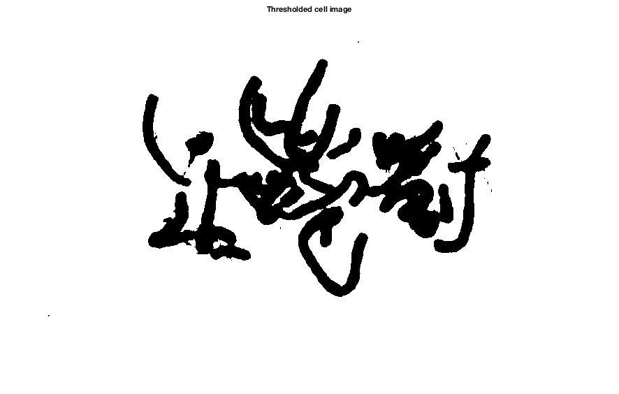
imshow(imbinarize(I))
title('Thresholded cell image')
If imbinarize handles this computation automatically, then why did we also provide a function called otsuthresh? The answer is that imbinarize takes an image as input, although Otsu's method does not require the original image, only the image's histogram. If you have a situation where you want to compute a threshold based only on a histogram, then you can call otsuthresh directly. That's why it is there.
To wrap up this week's discussion, I want to point out that a couple of blog readers recommended something called the Triangle method for automatic gray-scale image thresholding. If you want to try this for yourself, there is an implementation on the File Exchange. I have not had a chance yet to experiment with it.
Next time I'll talk about the algorithm used by imbinarize for locally adaptive thresholding.


コメント
コメントを残すには、ここ をクリックして MathWorks アカウントにサインインするか新しい MathWorks アカウントを作成します。