Image binarization – new R2016a functions

Posted by Steve Eddins, May 16, 2016

14 views (last 30 days) | 0 Likes | 3 comments

In my 09-May-2016 post, I described the Image Processing Toolbox functions im2bw and graythresh, which have been in the product for a long time. I also identified a few weaknesses in the functional designs:

The function im2bw uses a fixed threshold value (LEVEL) of 0.5 by default. Using graythresh to determine the threshold value automatically would be a more useful behavior most of the time.
If you don't need to save the value of LEVEL, then you end up calling the functions in a slightly awkward way, passing the input image to each of the two functions: bw = im2bw(I,graythresh(I))
Although Otsu's method really only needs to know the image histogram, you have to pass in the image itself to the graythresh function. This is awkward for some use cases, such as using the collective histogram of multiple images in a dataset to compute a single threshold.
Some users wanted to control the number of histogram bins used by graythresh, which does not have that as an option. (I forgot to mention this item in my previous post.)
There was no locally adaptive thresholding method in the toolbox.

For all of these reasons, the Image Processing Toolbox development undertook a redesign of binarization functionality for the R2016a release. The functional designs are different and the capabilities have been extended. We now encourage the use of a new family of functions:

Binarization using an automatically computed threshold value is now simpler. Instead of two function calls, im2bw(I,graythresh(I)), you can do it with one, imbinarize(I).

I = imread('cameraman.tif');
imshow(I)
xlabel('Cameraman image courtesy of MIT')

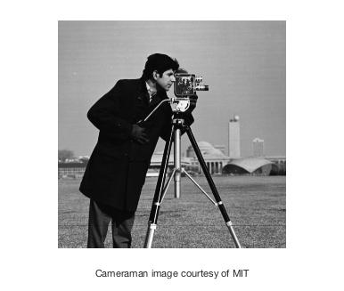
bw = imbinarize(I);
imshowpair(I,bw,'montage')

In addition to global thresholding, imbinarize can also do locally adaptive thresholding. Here is an example using an image with a mild illumination gradient from top to bottom.

I = imread('rice.png');
bw = imbinarize(I);
imshowpair(I,bw,'montage')
title('Original and global threshold')

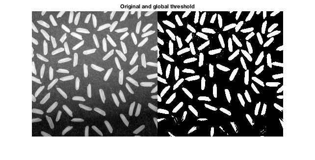
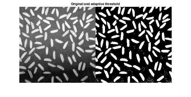
You can see that the rice grains at the bottom of the image are imperfectly segmented because they are in a darker portion of the image. Now switch to an adaptive threshold.

bw = imbinarize(I,'adaptive');
imshowpair(I,bw,'montage')
title('Original and adaptive threshold')

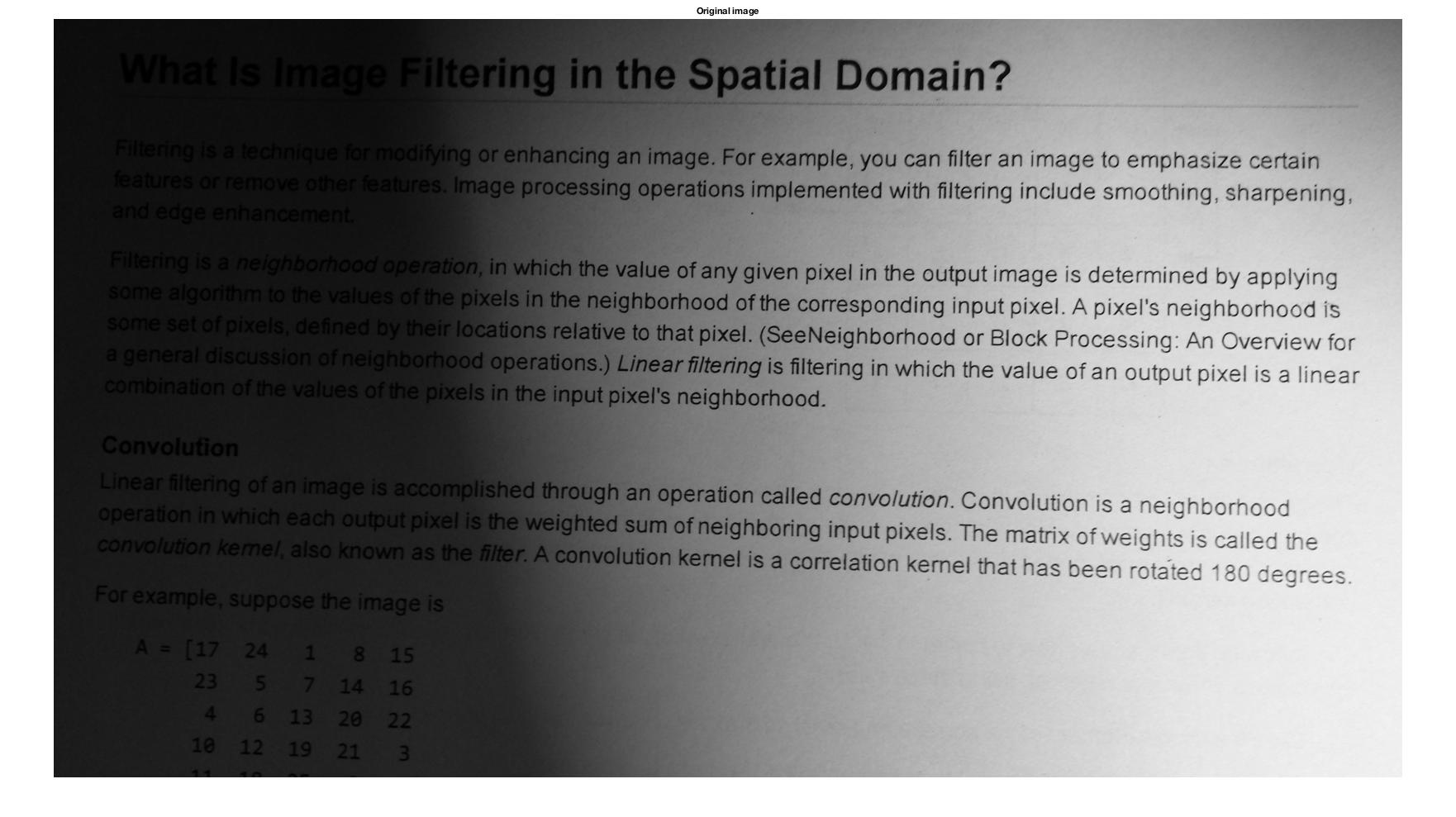
Here is a more extreme example of nonuniform illumination.

I = imread('printedtext.png');
imshow(I)
title('Original image')

bw = imbinarize(I);
imshow(bw)
title('Global threshold')

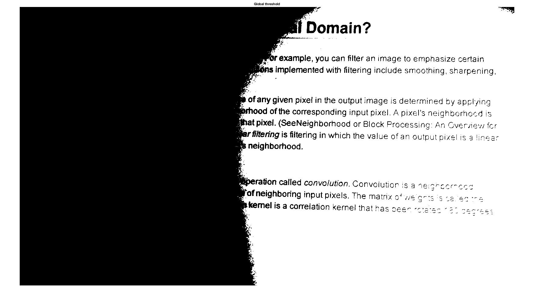
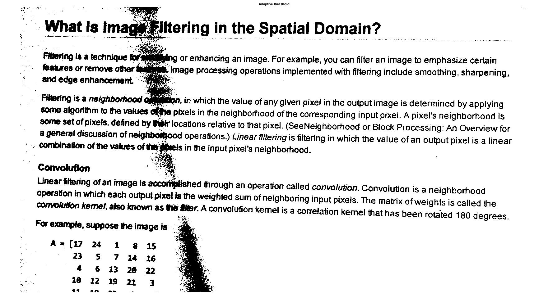
Let's see how using an adaptive threshold can improve the results. Before jumping into it, though, notice that the foreground pixels in this image are darker than the background, which is the opposite of the rice grains image above. The adaptive method works better if it knows whether to look for foreground pixels that are brighter or darker than the background. The optional parameter 'ForegroundPolarity' lets is specify that.

bw = imbinarize(I,'adaptive','ForegroundPolarity','dark');
imshow(bw)
title('Adaptive threshold')

The new functions otsuthresh and adaptthresh are for those who want to have more fine-grained control over the algorithms underlying the global and adaptive thresholding behavior of imbinarize. I'll talk about them next time.

Published with MATLAB® R2016a