 Cleve’s Corner: Cleve Moler on Mathematics and Computing
 The MATLAB Blog
 Guy on Simulink
 MATLAB Community
 Artificial Intelligence
 Developer Zone
 Stuart’s MATLAB Videos
 Behind the Headlines
 File Exchange Pick of the Week
 Hans on IoT
 Student Lounge
 MATLAB ユーザーコミュニティー
 Startups, Accelerators, & Entrepreneurs
 Autonomous Systems
 Quantitative Finance
 MATLAB Graphics and App Building
Pursuit Curves
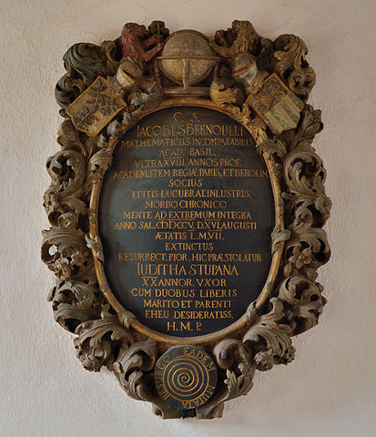
Here's an interesting snippet I learned while working on today's blog post: Mathematician Jacob Bernoulli asked for a logarithmic spiral to be engraved on his tombstone. Here's an example of a such a spiral.
theta = -6*pi:0.01:6*pi;
rho = 1.1.^theta;
polarplot(theta,rho)
rlim([0 max(rho)])
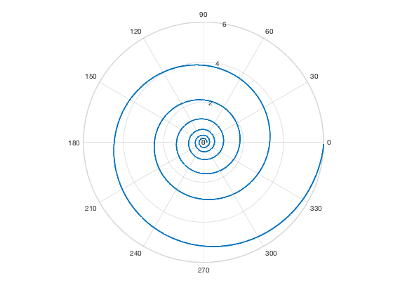
Sadly, the engravers of his tombstone apparently did not fully understand his request. They engraved a spiral, but it was not logarithmic.
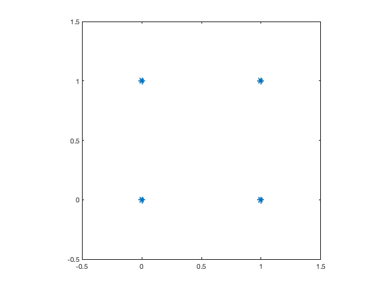
I came across the concept of logarithmic spirals while looking into something called pursuit curves. Here's an example, in the form of what is sometimes called the mice problem. Start by constructing P, a vector of four complex-valued points, so that they form the corners of a square in the complex plane.
P = [0 1 1+1i 1i];
plot(real(P),imag(P),'*')
axis equal
axis([-.5 1.5 -.5 1.5])
Now imagine that each of these "mice" is chasing the next one, always running directly toward it as is moves. To illustrate the basic idea, let's have the mice take a few fixed-length steps toward their targets.
P = [0 1 1+1i 1i];
step_size = 0.1;
Pt = P([2 3 4 1]);
V = Pt - P;
P = [P ; P + step_size*V];

% Second step
Pn = P(end,:);
Pt = Pn(end,[2 3 4 1]);
V = Pt - Pn;
P = [P ; Pn + step_size*V];

% Third step.
Pn = P(end,:);
Pt = Pn(end,[2 3 4 1]);
V = Pt - Pn;
P = [P ; Pn + step_size*V];

% Fourth step.
Pn = P(end,:);
Pt = Pn(end,[2 3 4 1]);
V = Pt - Pn;
P = [P ; Pn + step_size*V];
Now plot the original positions and steps taken by each mouse.
hold on
for k = 1:4
    plot(real(P(:,k)),imag(P(:,k)))
end
hold off
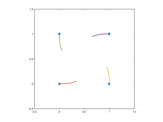
You get the idea, and you can see four spirals start to take shape.
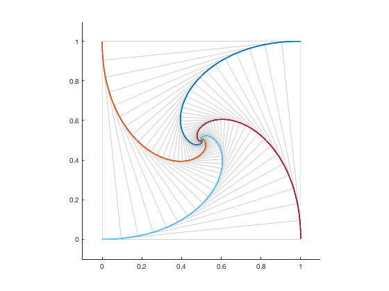
I've written a function, shown at the bottom of this post, that simulates and plots pursuit curves for any collection of starting points (mice). I chose to plot 1000 steps, with each step covering 1/100 of the remaining distance, so that the mice never quite catch their targets. The plotting function also plots the tangent lines every 10 steps. Here's the result for the four-mice-on-a-square starting configuration.
P = [0 1 1+1i 1i];
clf
plotPursuitCurves(P)
axis([-0.1 1.1 -0.1 1.1])
Logarithmic spiral curves have the interesting property that, when you scale them up by a constant factor, the curve remains the same, but rotated. We can get a sense of this property by zooming in on the plot. Let's zoom in by a factor of 100.
axis([0.495 0.505 0.495 0.505])
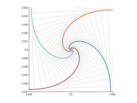
You can see that the curve's overall shape has not changed. It's just been rotated.
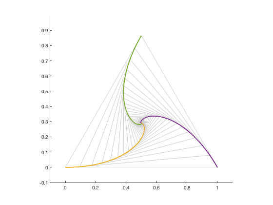
The function plotPursuitCurves lets us explore other starting configurations, such as a triangle.
clf
P1 = 0;
P2 = 1;
P3 = exp(1j*pi/3);
plotPursuitCurves([P1 P2 P3])
axis([-0.1 1.1 -0.1 1.0])
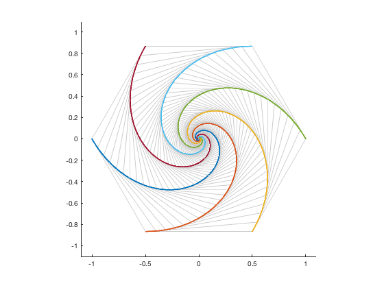
Or a hexagon.
clf
theta = 0:60:330;
P = cosd(theta) + 1i*sind(theta);
plotPursuitCurves(P)
axis([-1.1 1.1 -1.1 1.1])
We can even tinker with the select of targets. In this next example, the mice start at the vertices of a hexagon, but instead of chasing the next mouse over, they start out chasing other mice. We do this by reordering the vertices.
P2 = P([1 3 5 2 4 6]);
clf
plotPursuitCurves(P2)
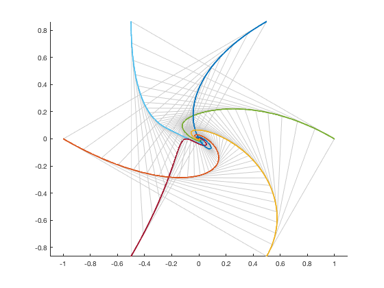
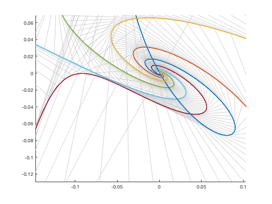
Those are some odd-looking curves. If we zoom in we can see why the curves evolve the way they do by examining the tangent lines. We can also see that the curves do appear to settle into a set of regular spirals, although I do not know whether this is a general property of such pursuit curves.
xlim([-0.147 0.103])
ylim([-0.129 0.069])
Do you like to explore mathematical visualizations like this? If you have a favorite, let us know in the comments.
function plotPursuitCurves(P)
P = reshape(P,1,[]);
N = length(P);
d = 0.01;
for k = 1:1000
    V = P(end,[(2:N) 1]) - P(end,:);
    P(end+1,:) = P(end,:) + d*V;
end

hold on
Q = P(:,[(2:N) 1]);
for k = 1:10:size(P,1)
    for m = 1:N
        T = [P(k,m) Q(k,m)];
        plot(real(T),imag(T),'LineWidth',0.5,'Color',[.8 .8 .8])
    end
end

for k = 1:N
    plot(real(P(:,k)),imag(P(:,k)))
end
hold off
axis equal
end


See Also
-

Happy Pi Day
Blogs
-

Magic Stars
Blogs


评论
要发表评论,请点击 此处 登录到您的 MathWorks 帐户或创建一个新帐户。