New Geometric Transformation Matrix Convention in R2022b

作者 Steve Eddins, November 1, 2022

12 次查看（过去 30 天） | 0 个赞 | 0 个评论

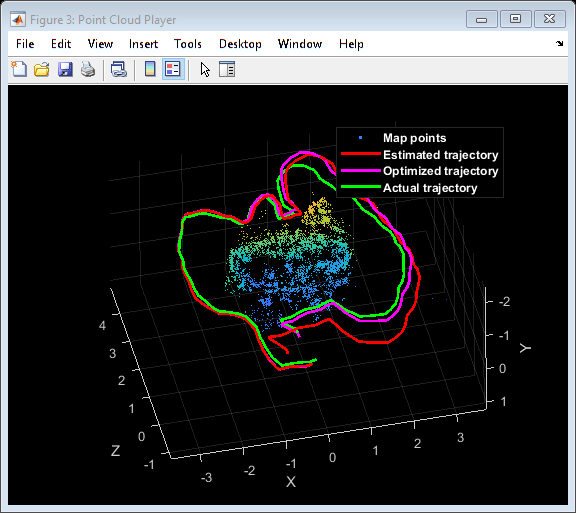
In the R2022b release, Image Processing Toolbox includes several new geometric transformation objects, such as rigidtform2d, affinetform3d, etc., that use the premultiply matrix convention instead of the postmultiply convention. Several other related toolbox functions, such as imregtform, now preferentially use these new objects. There are functions in the Computer Vision Toolbox and Lidar Toolbox that now use the premultiply convention and new objects. These changes also improve the design consistency with Robotics System Toolbox and Navigation Toolbox.

For the key information in the documentation, see:

In today's post, I'll explain how and why this all came about and what difference it makes to users.

Table of Contents

Affine Transformation Matrices
Competing Conventions
Deciding to Change the Convention
New Geometric Transformation Types
Using the New Types
Translation, Rigid, and Similarity Transformations
Transforming Points and Images
Related Toolboxes
Credits

Affine Transformation Matrices

The matrices in question define affine and projective transformations, including translations, rotations, rigid, and similarity transformations. I'll focus on affine transformations in the following discussion, but the same concepts apply to projective transformations.

For two dimensions, an affine transformation matrix is a $ 3 \times 3 $ matrix that maps a two-dimensional point, $ (u,v) $, using matrix multiplication, like this:

[xy1]=[abcdef001]×[uv1]=A×[uv1]

When the affine transformation is written as above, the third row of A is always [001]. Because the matrix appears before the vector it is multiplying, I'll call this the premultiply convention.

There's another way to write this operation. You can transpose everything, like this:

[xy1]=[uv1]×[ad0be0cf1]=[uv1]×B

In this form, the matrix appears after the vector, and so I'll call this the postmultiply convention. Note that A and B are related by matrix transposition: $ A = B^{T} $, and $ B = A^{T} $. 

Competing Conventions

The first Image Processing Toolbox release that included general-purpose geometric image transformation functions was developed from about 1999 to 2001. At that time, many of the most useful publications discussing the geometric transformation of images were in the computer graphics literature. Both of the matrix conventions, premultiply and postmultiply, were in use. Which convention you learned depended on which books and papers you read, or which graphics software framework you used, such as OpenGL or DirectX.

I was influenced at the time by the book Digital Image Warping, by George Wolberg, which used the postmultiply convention. I also thought that the postmultiply convention worked well with the usual MATLAB convention of representing P two-dimensional points as a $ P \times 2 $ matrix.

Because of these influences, the initial toolbox functions, maketform and imtransform, as well as the next generation of functions, imwarp and affine2d and others, used the postmultiply convention.

Within a few years, it became apparent that this design choice was confusing people. I mentioned the confusion in my 07-Feb-2006 blog post on affine geometric transformations.

Deciding to Change the Convention

In the years since 2001, the premultiply convention has become far more widely used than the postmultiply convention. The most popular sources of information, such as Wikipedia, use the premultiply convention. As a result, our use of the postmultiply convention was confusing many more people. We could see this confusion in many posts on MATLAB Answers, as well as in tech support requests. Developers on Image Processing Toolbox and Computer Vision Toolbox teams concluded that we should try to do something about it, even though it was likely to be difficult and time-consuming. The design effort began in spring 2021. The final push, in the winter and spring of this year, was a group effort (see below) involving developers, writers, and quality engineers on multiple teams.

New Geometric Transformation Types

The R2022b release of Image Processing Toolbox introduces these new types:

projtform2d - 2-D projective geometric transformation
affinetform2d - 2-D affine geometric transformation
simtform2d - 2-D similarity geometric transformation
rigidtform2d - 2-D rigid geometric transformation
transltform2d - 2-D translation geometric transformation
affinetform3d - 3-D affine geometric transformation
simtform3d - 3-D similarity geometric transformation
rigidtform3d - 3-D rigid geometric transformation
transltform3d - 3-D translation geometric transformation

We encourage everyone to start using these instead of the earlier set of types: projective2d, affine2d, rigid2d, affine3d, and rigid3d.

Using the New Types

When you make one of the new transformation types from a transformation matrix, use the premultiplication form. For an affine matrix in premultiplication form, the bottom row is [001].

A = [1.5 0 10; 0.1 2 15; 0 0 1]

A = 3×3
    1.5000         0   10.0000
    0.1000    2.0000   15.0000
         0         0    1.0000

tform = affinetform2d(A)

tform = 
  affinetform2d with properties:

    Dimensionality: 2
                 A: [3×3 double]

tform.A

ans = 3×3
    1.5000         0   10.0000
    0.1000    2.0000   15.0000
         0         0    1.0000

To ease the transition, the new types are intended to be interoperable, as much as possible, with code that was written for the old types. For example, let's take a look at the old function, affine2d:

T = A'

T = 3×3
    1.5000    0.1000         0
         0    2.0000         0
   10.0000   15.0000    1.0000

tform_affine2d = affine2d(T)

tform_affine2d = 
  affine2d with properties:

                 T: [3×3 double]
    Dimensionality: 2

tform_affine2d.T

ans = 3×3
    1.5000    0.1000         0
         0    2.0000         0
   10.0000   15.0000    1.0000

For the old types, the T property is the transformation matrix in postmultiply form. For the new types, the A property is the transformation matrix in premultiply form.

Although it is hidden, the new types also have a T property, and this property contains the transformation matrix in postmultiply form.

tform

tform = 
  affinetform2d with properties:

    Dimensionality: 2
                 A: [3×3 double]

tform.A

ans = 3×3
    1.5000         0  100.0000
    0.1000    2.0000   15.0000
         0         0    1.0000

tform.T

ans = 3×3
    1.5000    0.1000         0
         0    2.0000         0
  100.0000   15.0000    1.0000

This hidden property is there so that, if you have code that gets or sets the T property on the old type, you will be able to use the new type without changing that code. Setting or getting the T property will automatically set or get the corresponding A property.

tform.T(3,1) = 100;

tform.T

ans = 3×3
    1.5000    0.1000         0
         0    2.0000         0
  100.0000   15.0000    1.0000

tform.A

ans = 3×3
    1.5000         0  100.0000
    0.1000    2.0000   15.0000
         0         0    1.0000

Translation, Rigid, and Similarity Transformations

In addition to the generic affine transformation, the new types include the more specialized transformations translation, rigid, and similarity. You can create these using parameters that may be more intuitive than the affine transformation matrix. For example, a rigid transformation is a combination of rotation and translation, and so you can create a rigidtform2d object by specifying a rotation angle (in degrees) and a translation vector directly.

r_tform = rigidtform2d(45,[0.2 0.3])

r_tform = 
  rigidtform2d with properties:

    Dimensionality: 2
     RotationAngle: 45
       Translation: [0.2000 0.3000]
                 R: [2×2 double]
                 A: [3×3 double]

If you ask for R (the rotation matrix) or A (the affine transformation matrix), it is computed directly from the rotation and translation parameters.

r_tform.R

ans = 2×2
    0.7071   -0.7071
    0.7071    0.7071

r_tform.A

ans = 3×3
    0.7071   -0.7071    0.2000
    0.7071    0.7071    0.3000
         0         0    1.0000

You can change these matrices directly, but only if the result would be a valid rigid transformation. The following assignment, which only changes the horizontal translation offset, is permitted because the result is still a rigid transformation:

r_tform.A(1,3) = 0.25

r_tform = 
  rigidtform2d with properties:

    Dimensionality: 2
     RotationAngle: 45
       Translation: [0.2500 0.3000]
                 R: [2×2 double]
                 A: [3×3 double]

But if you try to change the upper-left $ 2 \times 2 $ submatrix so that it is not a rotation matrix, you'll get an error:

Transforming Points and Images

Transforming points and images works in the same way as with the old objects.

[x,y] = transformPointsForward(r_tform,2,3)

x = -0.4571
y = 3.8355

[u,v] = transformPointsInverse(r_tform,x,y)

u = 2
v = 3

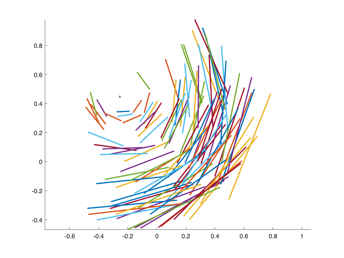
The following code generates 100 pairs of random points, transforms them using r_tform from above, and then plots line segments from the original points to the transformed ones.

xy = rand(100,2) - 0.5;

uv = transformPointsForward(r_tform,xy);

clf

hold on

for k = 1:size(xy,1)

    plot([xy(k,1) uv(k,1)],[xy(k,2) uv(k,2)])

end

hold off

axis equal

And imwarp interprets the new transformation types using the same syntax as before.

A = imread("peppers.png");

B = imwarp(A,r_tform);

imshow(B)

Related Toolboxes

These geometric transformation objects are widely used in several MathWorks toolboxes. There are currently 20 or so different documentation examples that use rigidtform3d. The examples are from these products:

Image Processing Toolbox
Computer Vision Toolbox
Automated Driving Toolbox
Lidar Toolbox

Here's a sampling:

Monocular Visual Simultaneous Localization and Mapping (vSLAM)

Build a Map with Lidar Odometry and Mapping (LOAM) Using Unreal Engine Simulation

Aerial Lidar SLAM Using FPFH Descriptors

Register Multimodal 3-D Medical Images

Credits

It took a big group effort, earlier this year, to make all the changes in Image Processing Toolbox, Computer Vision Toolbox, Automated Driving Toolbox, and Lidar Toolbox. The Image Processing Toolbox design and implementation, which I worked on, was relatively straightforward, but the Computer Vision Toolbox changes were extensive and quite complicated. Thanks go to Corey, Paola, and Qu for their implementation and design work. (Corey, I'm sorry that this project swallowed up your entire internship! I'm glad that you have officially joined the development team now.) Witek leaped in to help revise the Computer Vision Toolbox designs to incorporate lessons learned over the past several years. (Witek is co-author of the upcoming 2023 edition of Robotics, Vision, and Control: Fundamental Algorithms in MATLAB, which uses the premultiply convention.) From the Lidar Toolbox team, Kritika helped with design and implementation, and Hrishikesh updated some examples. 

Alex, thanks for being my Image Processing Toolbox design buddy; your experience was invaluable. Vignesh, thanks for advising me about code generation. Ashish, thanks for rescuing me at the very last minute with critical implementation help. Jessica did a wonderful job with the extensive documentation and example updates across all four products. And Abhi helped stage and qualify the final multiproduct integration under a tight deadline.