 Cleve’s Corner: Cleve Moler on Mathematics and Computing
 The MATLAB Blog
 Guy on Simulink
 MATLAB Community
 Artificial Intelligence
 Developer Zone
 Stuart’s MATLAB Videos
 Behind the Headlines
 File Exchange Pick of the Week
 Hans on IoT
 Student Lounge
 MATLAB ユーザーコミュニティー
 Startups, Accelerators, & Entrepreneurs
 Autonomous Systems
 Quantitative Finance
 MATLAB Graphics and App Building
Custom Vehicle Modeling using Simscape Language
Today, I am happy to introduce Andrea Casadio, he is a junior mechanical engineer and first-time guest in this blog. Andrea is going to describe his thesis work at Politecnico di Torino in which he developed Simscape™ libraries for vehicle modeling.
Thank you Andrea for providing the community with your work on MATLAB Central FileExchange.
– –
When I studied vehicle dynamics at university, I spent a lot of time modeling in Simulink®. What I did in fact was creating models based on fundamental equations trying to mimic actual systems. This approach became increasingly time consuming when I used more advanced system modeling approaches. Ultimately, I spent more time building vehicle models instead of developing and optimizing simulations.
At this point, I discovered Simscape. Simscape allows me to speed-up creating models of physical systems within the Simulink environment. Simscape blocks typically provide the functionality of a system of Simulink blocks within a single block.
Anyway, describing pros and cons of Simscape is not the scope of this post. So, let’s go with the work illustration!
At the beginning of my project, I discovered that default blocks of the Simscape Driveline library allow the simulation of longitudinal behavior only. The reason is that the tire blocks provided are based on mathematical models that take into account the longitudinal forces exchanged between tire and road. As expected, MathWorks offers functionality that allows to create custom components using the Simscape language.
For the reason above, the first target was to develop customized tire blocks based on more involved mathematical models like Pacejka ’89 and ’96, taking into account also the combination between lateral and longitudinal forces.

Fig. 1 – Example of a customized tire block
Lateral and longitudinal forces are functions of lateral and longitudinal tire slip, which depend on translational and rotational speed of the wheel. To develop such kinds of blocks it was necessary to use Simscape language to define:
- Conserving ports to transfer speed and force information;
- Declaration of domains, variables, parameters and equations.
Conserving ports are the interface with other Simscape components, on the example shown above there are “HX” and “HY” being the conserving ports defined on the mechanical translational domain. There is also “A” which is the conserving port defined on the mechanical rotational domain.
To validate the tire model, it was necessary to apply longitudinal and lateral motion to the tire model and it was possible to obtain the plots shown in Fig.2 and Fig.3.
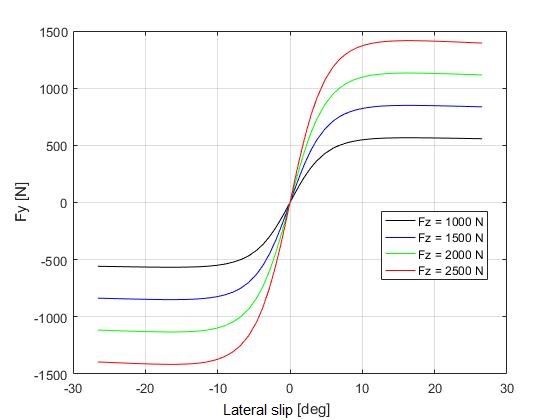
Fig.2 – Lateral force as a function of lateral slip at a different vertical loads – Pacejka ’89 model
Fig.2 displays the typical behavior of a tire when the longitudinal slip is zero (no braking or acceleration). The odd trend is a consequence of the Pacejka model. If you look at the block on Fig.1, there is no option to introduce a vertical load variable, this is introduced as a block parameter.
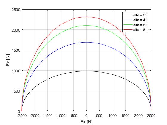
Fig.3 – Lateral force as a function of longitudinal force at a different lateral slip angles – Pacejka ’89 model
Applying different inputs to the block of Fig.1 it’s possible to obtain the graph on Fig.3, which displays how the lateral force between road and tire changes as a function of the longitudinal force for different lateral slip conditions (alpha). When the longitudinal force is zero, the lateral force is maximal. This is straightforward because tires’ grip on the corners is higher when the driver doesn’t apply brakes or throttle. The opposite condition is when the longitudinal force is maximal. In this case, the lateral force is zero. Even by common sense, you may agree that it is not a good idea to apply too much brakes or throttle on corners.
As done for tires, starting from a 3 degree of freedom (DOF) model of a vehicle, it was possible to develop a block describing vehicle body dynamics:
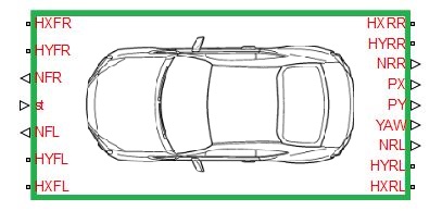
Fig.4 – 3 DOF Vehicle model
Here is a short description of the 3 DOF Vehicle model (Fig. 4):
- HXFR, HXFL, HXRR, HXRL are conserving ports defined on the mechanical translational domain. With these four connections it is possible to connect the vehicle body to other blocks (like tires), but only in the longitudinal direction. There is one port for every tire (FR means front right, RL means rear left, etc.)
- HYFR, HYFL, HYRR, HYRL are conserving ports defined on the mechanical translational domain. With these connections it is possible to connect the vehicle body to other blocks (like tires) in lateral direction
- NFR, NFL, NRR, NRL are the physical signal outputs representing the vertical loads. These ports are useful to make the block connectable with the one shown in Fig.1. In fact, the 3-DOF model doesn’t takes into account the load transfer during longitudinal or side acceleration. In this case, it’s considered being a constant value, depending on the load distribution of the vehicle on static condition without any kind of slope. ST is the physical input representing the steering angle
- PX, PT and YAW are three outputs representing the position along x, y and yaw. Yaw is the angle of rotation of the vehicle with respect to its vertical axis through the center of gravity (COG).
[Click on image to enlarge]
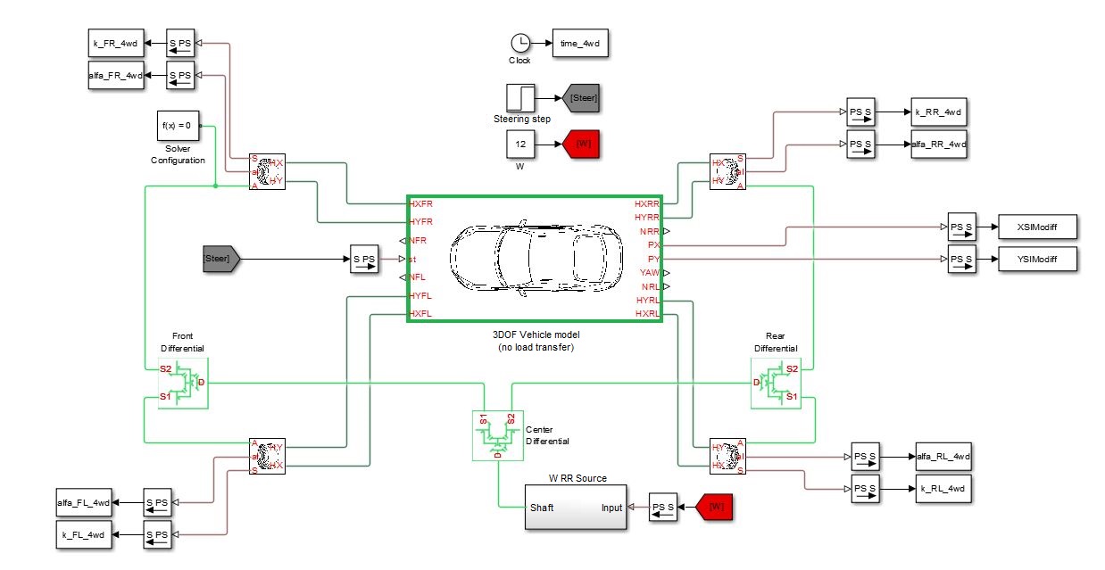
Fig.5 – A complete 3-DOF project – 4WD model with 3 differential
Systems like the one in Fig.5 allow to model vehicle behavior with:
- Input: steering wheel angle (ST);
- Output: coordinate of center of mass and yaw angle (PX, PY YAW).
To validate these blocks, four different configurations of a 4WD car with three differentials were defined, see Fig.6:
- All differentials opened
- Central differential locked
- Central and rear differential locked
- All differentials locked

Fig.6 – The four different configurations used to simulate the 3-DOF model
Saving on MATLAB workspace the center off mass coordinates, during the simulation, it was possible to plot the trajectory of the vehicle center of mass (see Fig.7). This plot shows, as expected, an increasing of under-steering behavior while the differentials have been locked.
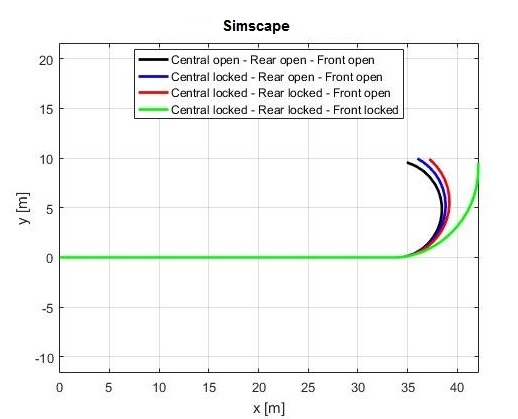
Fig.7 – Vehicle trajectories at different working conditions
Modeling vehicles with the previous defined customized blocks offers, in comparison with Simulink models, a cleaner representation of the system. However, it was not straightforward to define the vehicle dynamics block based on the equations of the physical system. No worries, as Christoph pointed out, I shared the material with you on MATLAB Central FileExchange.
Another alternative is using MathWorks’ multi-body simulation tool called Simscape Multibody™. Models look like the one shown on Fig.8 with its graphical representation in Fig.9.

[Click on image to enlarge]
Fig. 8 – A 6-DOF Vehicle model built with Simscape Multibody
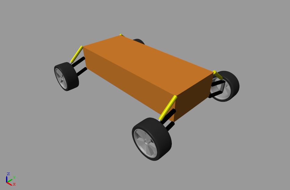
Fig.9 – A representation of the 6-DOF vehicle model
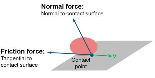
At the end, admittedly, it is hard to give compact advice on whether to use Simscape or Simscape Multibody. In very brief, Simscape Multibody will provide a graphic representation of your model automatically as you build the model. It will also allow you to model contact – find here a detailed introduction to contact modeling. In contrast to Simscape, these additional features will require more CPU time for solving system equations.
Let me refer you to a previous article in the racing lounge focusing on vehicle modeling. Especially, the modeling approach using Simscape Multibody will thoroughly discuss the pros and cons of Simscape Multibody. And even better, all models are provided on the MATLAB Central FileExchange.
If there is one key takeaway of my work, it is this: There are many opportunities to simulate vehicle models and investigate the influence of different suspension parameters. No matter whether you are working in Simulink, Simscape or Simscape Multibody, parameters can always be modified via the MATLAB workspace.
This work was an interesting opportunity to see the great potential of MATLAB when it comes to vehicle modeling. For sure, there are a lot of future possible implementations, for example the development of further tire models to consider the load transfer or the variation of characteristics wheel angles during the suspension travel. I would love to hear your feedback about my work.
Thank you MathWorks for the opportunity to publish in the racing lounge blog!


댓글
댓글을 남기려면 링크 를 클릭하여 MathWorks 계정에 로그인하거나 계정을 새로 만드십시오.