
Implicit Curves & Surfaces
Implicit Curves and Surfaces
In some earlier posts ( part1, part2) we explored how to draw parametric curves using MATLAB Graphics. Now lets turn our attention to implicit curves.
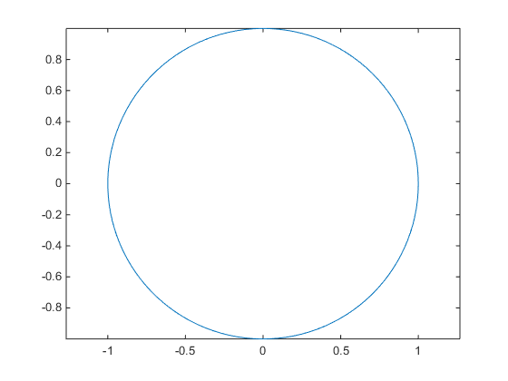
We know that the implicit equation for the unit circle is the following:

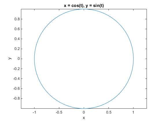
We can convert that into a parametric form, and then draw it using the techniques we learned earlier.
t = linspace(0,2*pi,120);
plot(cos(t),sin(t))
axis equal
But converting from implicit form to parametric form can be pretty complicated, even for a curve as simple as the unit circle. And there are implicit curves which don't have a parametric form. It'd be awfully nice if we could plot it directly without converting it to parametric form.
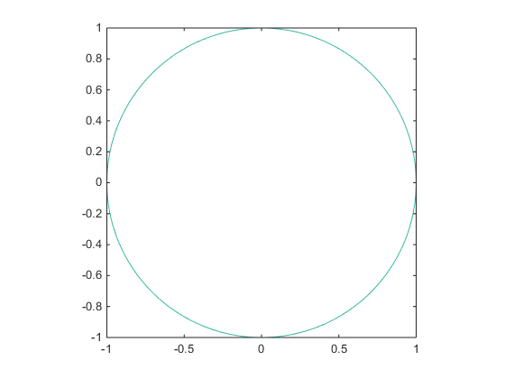
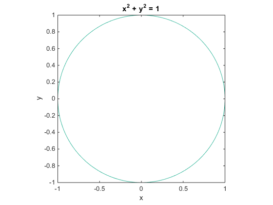
There is actually an easy way to do this, using the contour function. The basic idea is that we create a 2D array from the left hand side of the equation, and then contour it with one contour level which is equal to the right hand side of the equation.
[x,y] = meshgrid(linspace(-1,1,120));
contour(x,y,x.^2 + y.^2,'LevelList',1);
axis equal
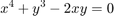
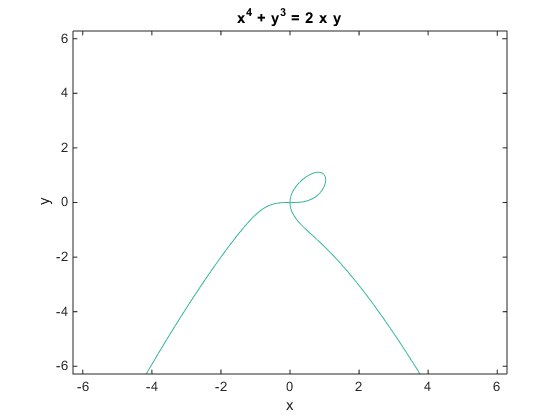
One problem with this approach is that it only works when the right hand side is a constant. To handle a function like this:

We'll have to transform it so that all of the non-constant terms are on the left:
[x,y] = meshgrid(linspace(-2*pi,2*pi,120));
contour(x,y,x.^4 + y.^3 - 2*x.*y,'LevelList',0);
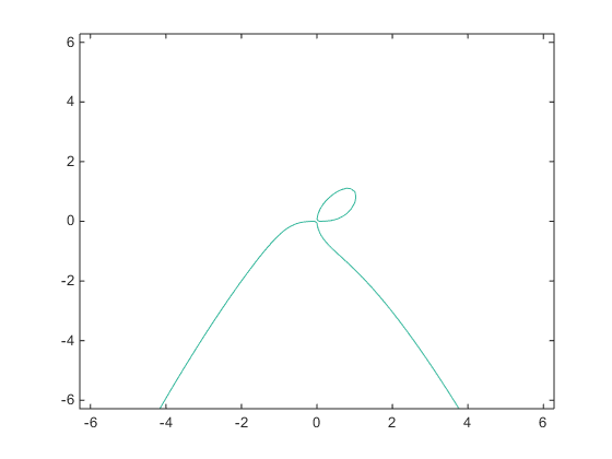
MATLAB Graphics actually provides a function which will take care of this for you. It's called ezplot.
ezplot('x^4 + y^3 = 2*x*y')
If you've ever used ezplot and looked at its return value, you might have noticed that it returns different types of objects for different types of equations. That's because it's doing exactly what I described above. If we call ezplot with a parametric equation, we get a Line object:
h = ezplot('cos(t)','sin(t)')
h =

  Line with properties:

              Color: [0 0.4470 0.7410]
          LineStyle: '-'
          LineWidth: 0.5000
             Marker: 'none'
         MarkerSize: 6
    MarkerFaceColor: 'none'
              XData: [1x300 double]
              YData: [1x300 double]
              ZData: [1x0 double]

  Use GET to show all properties
But if we call it with an implicit equation, we get a Contour object:
h = ezplot('x^2 + y^2 = 1',[-1 1])
axis equal
h =

  Contour with properties:

    LineColor: 'flat'
    LineStyle: '-'
    LineWidth: 0.5000
         Fill: 'off'
    LevelList: 0
        XData: [1x250 double]
        YData: [250x1 double]
        ZData: [250x250 double]

  Use GET to show all properties
What about implicit equations in 3D? Neither the ezplot function or its companion ezsurf can do this. But now that we know how ezplot works for 2D implicit equations, we can use the same technique. We just need to switch from the contour function to the isosurface function. The isosurface function does for a 3D array what the contour function does for a 2D array.
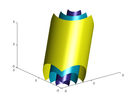
For example, Guillermo asked on MATLAB Answers how to draw the following surface.

Where R is a positive integer.
We can generate a 3D grid of the left hand side using ndgrid.
[y,x,z] = ndgrid(linspace(-5,5,64));
f = (y-z).^2 + (z-x).^2 + (x-y).^2;
Once we have that, we can use the isosurface function to figure out where that function is equal to the right hand side for various values of R.
cla reset
r = 1;
isosurface(x,y,z,f,3*r^2)
r = 2;
isosurface(x,y,z,f,3*r^2)
r = 3;
isosurface(x,y,z,f,3*r^2)
view(3)
camlight
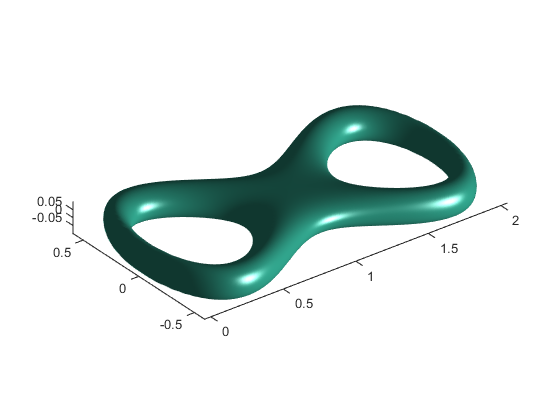
Here's a slightly more complex implicit surface from this Stack Exchange post.

[y,x,z] = ndgrid(linspace(-.75,.75,100),linspace(-.1,2.1,100),linspace(-.2,.2,100));
f = (x.*(x-1).^2.*(x-2) + y.^2).^2 + z.^2;
cla
isosurface(x,y,z,f,.01);
view(3);
camlight
axis equal
But some implicit surfaces are very complex and can be rather tricky to render. One of my favorite challenges are the famous Barth surfaces. For example, the equation for the sextic is the following:

Here's a picture I made of it for w=1.
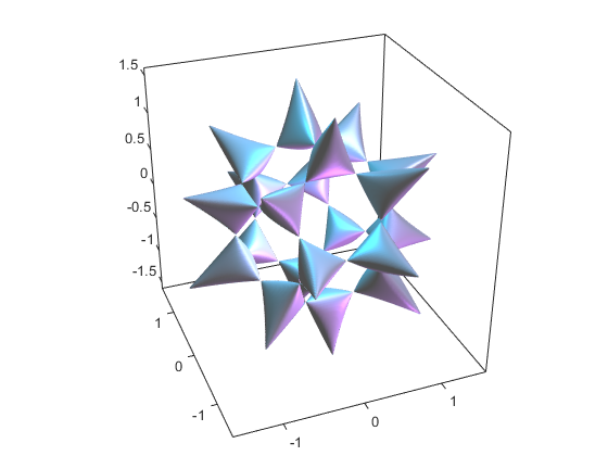
Can you create a better picture of this challenging surface or one of its relatives?
- Category:
- Geometry

