The QR Algorithm Computes Eigenvalues and Singular Values
The QR algorithm is one of the world's most successful algorithms. We can use animated gifs to illustrate three variants of the algorithm, one for computing the eigenvalues of a nonsymmetric matrix, one for a symmetric matrix, and one for the singular values of a rectangular matrix. In all three cases, the QR iteration itself is preceded by a reduction to a compact form. All transformations are orthogonal similarities using Givens and Householder transformations. These are numerically stable, preserve eigenvalues, and preserve any symmetry.
 The initial reduction uses n-2 Householder similarites to introduce zeroes below the subdiagonal a column at a time. The result is known as a Hessenberg matrix (don't let spell-checkers change that to Heisenberg matrix.)
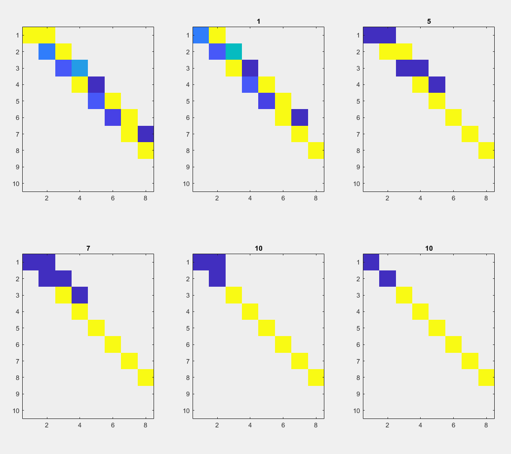
 Now the QR algorithm gradually reduces most subdiagonal elements to roundoff level, so they can be set to zero. The corresponding diagonal element is an eigenvalue. The iteration count is shown in the title. The element below the diagonal in the last row is the initial target; it requires four iterations. The next two rows require three iterations each. The remaining subdiagonals require just one or two iterations each.
 All this is done with real arithmetic, although a real, nonsymmetric matrix may have complex eigenvalues. So the final matrix may have 2-by-2 bumps on the diagonal. This example has one bump in rows 3 and 4. The eigenvalues of a bump are a complex conjugate pair of eigenvalues of the input matrix. All the other diagonal elements are real eigenvalues of the input matrix.
 The computed eigenvalues are:
 By symmetry the six Householders that zero the columns also zero the rows.
 Now the QR iteration works on just two vectors, the diagonal and the off-diagonal.
 The limit is the diagonal containing the eigenvalues.

 Use a Householder operating from the left to zero a column and then another Householder operating from the right to zero most of a row.
 Now a two-sided QR iteration reduces the off diagonal to negligible size.
 The resulting diagonal contains the singular values.

Contents
The starting matrix for all three variants is based on flipping the Rosser matrix.A = fliplr(rosser)
A =

    29   -49   -52    -8   407  -192   196   611
   -44    -8   -43   -71  -192   113   899   196
    52     8    49    61   196   899   113  -192
   -23    59    44     8   611   196  -192   407
   208   208  -599   411     8    61   -71    -8
   208   208   411  -599    44    49   -43   -52
  -911    99   208   208    59     8    -8   -49
    99  -911   208   208   -23    52   -44    29
Nonsymmetric eigenvalues
Here is a static picture of the starting matrix. Notice that it is not symmetric. The initial reduction uses n-2 Householder similarites to introduce zeroes below the subdiagonal a column at a time. The result is known as a Hessenberg matrix (don't let spell-checkers change that to Heisenberg matrix.)
 Now the QR algorithm gradually reduces most subdiagonal elements to roundoff level, so they can be set to zero. The corresponding diagonal element is an eigenvalue. The iteration count is shown in the title. The element below the diagonal in the last row is the initial target; it requires four iterations. The next two rows require three iterations each. The remaining subdiagonals require just one or two iterations each.
 All this is done with real arithmetic, although a real, nonsymmetric matrix may have complex eigenvalues. So the final matrix may have 2-by-2 bumps on the diagonal. This example has one bump in rows 3 and 4. The eigenvalues of a bump are a complex conjugate pair of eigenvalues of the input matrix. All the other diagonal elements are real eigenvalues of the input matrix.
 The computed eigenvalues are:
       -1010.9
        1017.3
       -14.529 + 903.74i
       -14.529 - 903.74i
         206.9
       -30.004
        1.7094
     5.614e-13
Symmetric eigenvalues
A symmetric matrix isS = (A + A')/2; fprintf([repmat(' %7.1f',1,8) '\n'],S)
    29.0   -46.5     0.0   -15.5   307.5     8.0  -357.5   355.0
   -46.5    -8.0   -17.5    -6.0     8.0   160.5   499.0  -357.5
     0.0   -17.5    49.0    52.5  -201.5   655.0   160.5     8.0
   -15.5    -6.0    52.5     8.0   511.0  -201.5     8.0   307.5
   307.5     8.0  -201.5   511.0     8.0    52.5    -6.0   -15.5
     8.0   160.5   655.0  -201.5    52.5    49.0   -17.5     0.0
  -357.5   499.0   160.5     8.0    -6.0   -17.5    -8.0   -46.5
   355.0  -357.5     8.0   307.5   -15.5     0.0   -46.5    29.0
Here is the static picture. (The computation is done on half of the matrix, but we show the entire array.)
 By symmetry the six Householders that zero the columns also zero the rows.
 Now the QR iteration works on just two vectors, the diagonal and the off-diagonal.
 The limit is the diagonal containing the eigenvalues.

       -1010.9
        1017.4
       -558.86
       -481.89
        -86.32
         109.7
         662.7
        504.27
SVD
Make our test matrix rectangular by inserting a couple of rows of the identity matrix.I = eye(8,8); A = [A(1:4,:); I(1,:); A(5:8,:); I(2,:)]
A =

    29   -49   -52    -8   407  -192   196   611
   -44    -8   -43   -71  -192   113   899   196
    52     8    49    61   196   899   113  -192
   -23    59    44     8   611   196  -192   407
     1     0     0     0     0     0     0     0
   208   208  -599   411     8    61   -71    -8
   208   208   411  -599    44    49   -43   -52
  -911    99   208   208    59     8    -8   -49
    99  -911   208   208   -23    52   -44    29
     0     1     0     0     0     0     0     0
 Use a Householder operating from the left to zero a column and then another Householder operating from the right to zero most of a row.
 Now a two-sided QR iteration reduces the off diagonal to negligible size.
 The resulting diagonal contains the singular values.

       0.44272
       0.13184
          1000
          1000
        1019.9
          1020
          1020
          1020


コメント
コメントを残すには、ここ をクリックして MathWorks アカウントにサインインするか新しい MathWorks アカウントを作成します。