
Kuramoto Model of Synchronized Oscillators
Fireflies on a summer evening, pacemaker cells, neurons in the brain, a flock of starlings in flight, pendulum clocks mounted on a common wall, bizarre chemical reactions, alternating currents in a power grid, oscillations in SQUIDs (superconducting quantum interference devices). These are all examples of synchronized oscillators.
The Kuramoto model is a nonlinear dynamic system of coupled oscillators that initially have random natural frequencies and phases. If the coupling is strong enough, the system will evolve to one with all oscillators in phase.
Contents
Yoshiki Kuramoto
Yoshiki Kuramoto is a Professor Emeritus of physics at Kyoto University. He was born in 1940 and published the first paper about this model in 1974. He was quite surprised when his model turned out to abstractly describe the dynamics of so many different physical systems. Here is a YouTube video made in 2015 of him reminiscing about the model.
Kuramoto model
The Kuramoto model is a system of $n$ ordinary differential equations
$$\dot{\theta_k} = \omega_k + \frac{\kappa}{n}\sum_{j=1}^n {\sin{(\theta_j-\theta_k)}}, \ k = 1,....,n$$
Here $\theta_k(t)$ is a real-valued function of $t$ describing the state of the $k$-th oscillator, $\omega_k$ is the natural frequency of the $k$-th oscillator and the real scalar $\kappa$ is the strength of the coupling between the oscillators.
When $\kappa = 0$, the equations are linear and the oscillators are independent.
$$\theta_k(t)= \omega_k t$$
When $\kappa$ is increased beyond a critical point, the nonlinear term forces the phases of all the oscillators to approach a common limit.
Kuramoto app
Here is the help entry for my kuramoto program.
help kuramoto_
Kuramoto. Kuramoto's model of synchronizing oscillators.
kuramoto(n) has n oscillators. Default is n = 100.
The model is a system of n ordinary differential equations.
The k-th equation is
(d/dt) theta_k = omega_k + kappa/n*sum_j(sin(theta_j-theta_k))
theta_k is the phase of the k-th oscillator,
omega_k is the intrinsic frequency of the k-th oscillator,
kappa is a scalar coupling parameter.
Initially, theta is distributed uniformly in the interval [0,2*pi]
and omega is distributed uniformly in the interval [1-b,1+b]
where b is a parameter called breadth.
The angular velocities of exp(i*theta) are color coded with blues
for the fastest, yellows for the slowest, and greens in between.
The display radius of exp(i*theta) is distributed normally with
mean 1 and standard deviation w where w is a parameter called width.
This is purely for visual effect and has no influence on the dynamics.
Setting width to zero puts all the oscillators on the unit circle.
The interface allows control of n, kappa, the speed of the ode solver,
breadth and width.
An alternate display mode, called "rotate", is a frame of reference
rotating with angular velocity psi, the average of the thetas.
A rotating arrow has length |z| where
|z|*exp(i*psi) = 1/n*sum_k(exp(i*theta_k)).
|z| = 0 indicates no synchronization, |z| = 1 is complete synchronization.
Animations
I have made five animated gifs showing the program in action. Each animation is a slight variation of the others. I hope your browser or viewer is showing them moving together. If that isn't happening, let us know in the comments what system you are using.
kappa = 0
Here are the default settings of the controls, including kappa = 0. The oscillators are each moving at their natural frequency. There is no synchronization.
kappa = 0.50
Bump the coupling parameter up to kappa = 0.50. This forces the oscillators to move to a common frequency. The order parameter arrow grows to its full length. Near the end of this sample the slowest yellow is trying to catch up with the others.
rotate on
You can see this better in the rotating coordinates that I have called "rotate". The blues, which are faster than the average, are moving in one direction, while the slower yellows are moving in the opposite direction.
kappa = 0.12
Turn the coupling parameter back down to 0.12. This is near the threshold value that initiates synchronization. The arrow is growing slowly, but we stop before it reaches full length.
width = 0
Set the width to zero. This is the same action as the previous animation but confined to the circle. It's harder to see what's happening.
One-liner
The code for Kuramoto's system of odes is a MATLAB™ one-liner.
   function theta_dot = ode(~,theta)
       theta_dot = omega + kappa/n*sum(sin(theta-theta'))';
   end
n and kappa are real scalars. omega and theta are real column vectors of length n. Singleton expansion makes theta-theta' into an n -by- n matrix with elements theta(j)-theta(k). The sum produces a row vector and the final transpose makes the result a column vector.
Software
I have submitted kuramoto to the MATLAB Central File Exchange. Here is the link. I have also included it in version 4.60 of Cleve's Laboratory.
References
Wikipedia, Kuramoto model, https://en.wikipedia.org/wiki/Kuramoto_model.
Dirk Brockman and Steven Strogatz, "Ride my Kuramotocycle", https://www.complexity-explorables.org/explorables/ride-my-kuramotocycle.


Comments
To leave a comment, please click here to sign in to your MathWorks Account or create a new one.