 Cleve’s Corner: Cleve Moler on Mathematics and Computing
 The MATLAB Blog
 Guy on Simulink
 MATLAB Community
 Artificial Intelligence
 Developer Zone
 Stuart’s MATLAB Videos
 Behind the Headlines
 File Exchange Pick of the Week
 Hans on IoT
 Student Lounge
 MATLAB ユーザーコミュニティー
 Startups, Accelerators, & Entrepreneurs
 Autonomous Systems
 Quantitative Finance
 MATLAB Graphics and App Building
Gil Strang and the CR Matrix Factorization
My friend Gil Strang is known for his lectures from MIT course 18.06, Linear Algebra, which are available on MIT OpenCourseWare. He is now describing a new approach to the subject with a series of videos, A 2020 Vision of Linear Algebra. This vision is featured in a new book, Linear Algebra for Everyone.
Contents
The CR factorization
Gil's approach will be familiar to MATLAB users and to readers of this blog. The key components are matrix factorizations -- LU, QR, eigenvalues and SVD. But before he gets to those, Gil likes to start with a more fundamental factorization, A = C*R, that expresses any matrix as a product of a matrix that describes its Column space and a matrix that describes its Row space.
For example, perhaps the first 3-by-3 matrix anybody writes down is
A =
      1     2     3
      4     5     6
      7     8     9
Notice that the middle column is the average of the first and last columns, so the most obvious CR factorization is
C =
      1     3
      4     6
      7     9
R =
      1     0.5     0
      0     0.5     1
However, this not the only possible CR factorization. For another one, keep reading.
The CR factorization works beautifully for the matrices encountered in any introduction to linear algebra. These matrices are not too large, and their entries are usually small integers. There are no errors in the input data, and none are expected in the subsequent computation. But, as Gil freely admits, the CR factorization is not a contender for any serious technical use.
The factorization A = C*R is rank_revealing. The number of columns in C must be the same as the number of rows in R. The smallest number of columns for which the product C*R reproduces A is defined to be the rank of A. So here, in the first few days of the course, a fundamental concept is introduced. It goes by many names -- low rank approximation, model reduction, principal components analysis -- and it pervades modern matrix computation. Look under the hood in many AI and ML success stories and you may well find something akin to a CR factorization.
Reduced row echelon form
I think Gil was pleased when he realized that a good choice for R was an old friend, the reduced row echelon form, featured in linear algebra textbooks for decades. Since you've probably forgotten them, or never knew them, these are the requirements for a matrix to be in reduced row echelon form.
- The first nonzero entry is any nonzero row is a 1, called the leading 1.
- All of the other elements in a column containing a leading 1 are zero.
- Each leading 1 occurs later in its row than the leading 1's in earlier rows.
- Any all zero rows are below the nonzero ones. (We will soon delete them.)
In the above example, the matrix R is not in reduced row echelon form, because the first nonzero element in the second row is not a 1.
The "reduced" in the name refers to the zeros above each leading 1. The algorithm for computing the reduced form is known as Gauss-Jordan elimination. Its computational complexity is 50 percent more than conventional Gaussian elimination.
An identity matrix is in reduced row echelon form, so if A is square and invertible, or, in general, has n linearly independent columns, then A = C and R is the n -by- n identity. We expect rank deficient matrices to have more interesting CR factorizations.
One important fact about the reduced form is that it is unique. No matter how you compute it, there is exactly one matrix that meets all the criteria in our bulleted list. So, if we require R to be in reduced row echelon form, the CR factorization of any matrix is unique.
You can see the source code for the MATLAB rref with
type rref
One of the 80 functions in my original pre-MathWorks Fortran MATLAB was rref, although it didn't come from LINPACK or EISPACK.
function cr
Since MATLAB already has rref, it took me five minutes, and as many executable lines, to write this function.
function [C,R] = cr(A)
    R = rref(A);
    j = find(sum(double(R)~=0)==1);    % Indices of leading ones.
    r = length(j);                     % r = rank.
    R = R(1:r,:);                      % Delete all zero rows so R(:,j) == eye(r).
    C = A(:,j);
end
Actually, I originally had only four executable lines since rref also provides the indices j of the columns containing the leading 1's. But that is only if the class of A is single or double. If A is a sym, the Symbolic Math Toolbox makes me compute j from R.
The columns of C are the first r linearly independent columns of A. All the linear combination action comes from R.
The length of j, the rank, is the most important quantity this function computes. Everything else depends upon it.
For our example, the above A,
[C,R] = cr(A)
C =
      1     2
      4     5
      7     8
R =
      1     0    -1
      0     1     2
Now C is the first two columns of A and R is in reduced row echelon form (without the zero row).
magic(4*k)
My favorite rank deficient matrices are the MATLAB versions of magic squares with size that is a multiple of four. All of them, no matter how large, have rank 3. Let's find the CR factorization of magic(8).
   A = magic(8)
   [C,R] = cr(A)
A =
    64     2     3    61    60     6     7    57
     9    55    54    12    13    51    50    16
    17    47    46    20    21    43    42    24
    40    26    27    37    36    30    31    33
    32    34    35    29    28    38    39    25
    41    23    22    44    45    19    18    48
    49    15    14    52    53    11    10    56
     8    58    59     5     4    62    63     1
C =
    64     2     3
     9    55    54
    17    47    46
    40    26    27
    32    34    35
    41    23    22
    49    15    14
     8    58    59
R =
     1     0     0     1     1     0     0     1
     0     1     0     3     4    -3    -4     7
     0     0     1    -3    -4     4     5    -7
The fact that C has three columns and R has three rows indicates that the rank of A is 3. The columns of C are the first three columns of A. The first three rows and columns of R form the 3-by-3 identity matrix. The rest of R contains the coefficients that generate all of A from its first three columns.
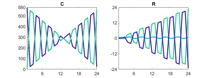
The patterns that we see in C and R come from the algorithm that generates magic squares of order 4*k. Here are plots of C and R for the 24-by-24 magic square.
A = magic(24)
[C,R] = cr(A)
plot(C)
plot(R)
west0479
We don't expect the CR factorization to work on larger matrices with inexact entries, but let's try it anyway.
The matrix west0479 has a venerable history. In 1983, Art Westerberg, a chemical engineering professor at Carnegie Mellon, contributed eleven matrices extracted from modelling chemical engineering plants to the Harwell-Boeing Sparse Matrix collection. One of these matrices, west0479, is a model of an eight-stage distillation column. It is 479-by-479 and has 1887 nonzero entries.
In 1990, when we introduced sparse matrices in MATLAB, we included west0479 in the demos directory. It has been available in all subsequent releases.
   clear
   load west0479
   whos
  Name            Size             Bytes  Class     Attributes

  west0479      479x479            34032  double    sparse
Today, Google finds 71 web pages that mention west0479. I stopped counting the number of images on the web that it has generated.
Our cr will work on the sparse matrix, but it is faster to convert it to full first.
   A = full(west0479);
   [C,R] = cr(A);
   r = size(C,2)
r =
   479
So, cr decides this matrix has full rank and returns with C = A and R = I. Not very useful.
Dueling rref
Upon closer examination, we find rref has an optional second input argument named tol. Let's see if that will help us compute a more useful CR factorization. The help entry says
[R,jb] = rref(A,TOL) uses the given tolerance in the rank tests.
I wrote rref years ago and I must say now that this description is not very specific. It should say that any column encountered during the reduction whose largest element is less than or equal to tol is replaced by all zeros.
The largest element in west0479 is about 3.2e5 and the smallest nonzero is 1.0e-6, so the elements range over eleven orders of magnitude. It turns out that the matrix has many columns with only two nonzero entries, the largest of which is +1 or -1. So, any tol larger than 1 causes rref to ignore those columns. And any tol less than 1 includes those columns. This leads to excessive sparse matrix fill-in.
This animation compares rref with tol = 0.99 to rref with tol = 1.01. Watch the nonzero counts in the spy plots. The count for tol = 0.99 rises to over seven times the count in the original matrix, before it drops somewhat at the end. The final nonzero count for tol = 1.01 is less than the starting nnz. That is not a good sign.
Ultimately, neither value of tol produces a CR factorization which is close to the original matrix, and no other values do any better. As we expected, CR is just not useful here.


コメント
コメントを残すには、ここ をクリックして MathWorks アカウントにサインインするか新しい MathWorks アカウントを作成します。