
Continued Fractions and Computations
Today's guest article is by Wesley Hamilton, a STEM Outreach engineer here at MathWorks. See his earlier piece on solving Sudoku puzzles.
In this blog post we'll explore the fascinating world of continued fractions, like $ \sqrt{2} = 1 + \frac{1}{2 + \frac{1}{2 + \frac{1}{2 + \cdots}}} $. While these objects have been studied for several centuries, their presence in modern math classes is relatively rare (unless you're studying number theory, probably). One of the historical uses of these objects has been computing rational approximations of irrational numbers, such as the 5th century approximations for π of $ \frac{22}{7} $ and $ \frac{355}{113} $ by Chinese astronomer Zu Chongzhi. Here, we'll focus on something even less prevalent: their computational aspects. The goal is to start exploring statistical properties of continued fractions, generating conjectures, and then pointing to several topics that can serve as computational playgrounds to get one's hands dirty and explore even more.
Before defining what a continued fraction even is, we'll start by defining a few "important" numbers to use as examples throughout. Next we'll define continued fractions and compute some by hand, before introducing the computational algorithm to compute these things. Afterwards we'll explore their statistical properties, before discussing some conjectures and neat facts, and round out the discussion by including links to other interesting computational topics to explore.
Table of Contents
Some Numbers
So that we have a rich class of examples, let's set up a few "important" numbers to use throughout the rest of this blog. Some of the numbers are important in some area(s) of math, though the whole collection should give us a nice, diverse set of examples to explore with. Also some of the names used are likely not standard, but describe how the numbers are constructed fairly well.
First, let's set up some parameters that'll determine the precision we'll be using throughout, along with a random number seed to ensure reproducibility no matter which machine (and when) these examples are run.
d = 10000; %set the computational precision "very" high
rng(1); %set the seed for the random number generator
And with that, let's set up our collection of numbers. For those interested in learning about each number, check out the code block at the end of this post. If you're content with knowing these are just being used as examples, feel free to skip seeing the definitions.
[num1, num2, num3, num4, num5, num6] = generateExamples(d);
Continued Fractions
So what exactly is a continued fraction? As the name implies, a continued fraction is a fraction that continues. What are fractions that don't continue? Most fractions you might think of, such as $ \frac{11}{13} $.
This isn't the only way to write this fraction though. One way, using Egyptian fractions, is $ \frac{11}{13} = \frac{1}{2} + \frac{1}{3} + \frac{1}{78} $, which we can verify using MATLAB's Symbolic Math Toolbox (which will also be used significantly later on):
eFrac = sym(1/2) + sym(1/3) + sym(1/78)
Another way is $ \frac{11}{13} = \frac{1}{1 + \frac{1}{ 5 + \frac{1}{2}}} $. We can check this just as we did above:
cFrac = 1/(1 + 1/(5 + sym(1/2)))
This is what we call a finite (simple) continued fraction: continued fraction because it continues, finite because there are finitely many terms, and simple because the numerators that appear are all 1. We also note that all of the coefficients we want should be positive integers; variations with negative integers also exist and the resulting continued fractions will have different properties.
This begs two natural questions:
- Are there continued fractions that have infinitely many terms?
- Are there continued fractions with numerators other than 1?
Yes and yes, which we'll demonstrate by example:
- The golden ratio $ \phi = \frac{1 + \sqrt{5}}{2} = 1+ \frac{1}{1 + \frac{1}{1 + \cdots}} \approx 1.618... $,
- $ \frac{4}{\pi} = 1 + \frac{1^2}{2 + \frac{3^2}{2 + \frac{5^2}{2 + \cdots}}} \approx 1.2732... $.
In this post we'll focus on infinite continued fractions, which we'll refer to as continued fractions for simplicity. Likewise, we won't touch on non-simple continued fractions, but rest assured they exist and often express interesting patterns and are fascinating mathematical objects to explore; for simplicity, whenever we say continued fraction we're talking about a simple continued fraction.
So how does one compute the continued fraction for a number? The general algorithm is a sort of Euclid's algorithm, wherein we take off the integer portion of a number, invert the fraction, and repeat. Let's see how this works with $ \frac{11}{13} $:
- $ \frac{11}{13} $ has no integer part, so we have $ \frac{11}{13} = 0 + \frac{11}{13} $.
- Next we invert the fractional part of the last expression, giving $ \frac{11}{13} = 0 + \frac{1}{\frac{13}{11}} $.
- For the newest "denominator", we repeat the process of taking out an integer part: since $ \frac{13}{11} = 1 + \frac{2}{11} $, we get $ \frac{11}{13} = 0 + \frac{1}{1 + \frac{2}{11}} $.
- Having isolated the integer part, we now invert the new fractional part $ \frac{2}{11} $, giving $ \frac{11}{13} = 0 + \frac{1}{1 + \frac{1}{\frac{11}{2}}} $.
- Since $ \frac{11}{2} = 5 + \frac{1}{2} $, we substitute this in to get the continued fraction $ \frac{11}{13} = 0 + \frac{1}{1 + \frac{1}{5 + \frac{1}{2}}} $.
It shouldn't be too surprising that any finite continued fraction corresponds to a rational number (just apply the algorithm backwards from the end of the continued fraction), but it may not be obvious that every rational number has a finite continued fraction. As a comparison, the decimal representation of $ \frac{1}{2} $ is $ 0.5 $, while the decimal representation of $ \frac{1}{3} $ is $ 0.333... $. It turns out that for continued fractions, there will be infinitely many coefficients if the number is irrational, and likewise if the number is irrational its continued fraction will have infinitely coefficients.
Infinite Continued Fractions
We've already seen one example of an infinite continued fraction, $ \phi = 1+ \frac{1}{1 + \frac{1}{1 + \cdots}} $. There are two ways to find the coefficients: one involves the algorithm from above, while the other leverages the fact that ϕ is a solution to $ 0 = \phi^2 - \phi - 1 $. Let's see both methods in action:
- Using the approximation $ \phi =1.618033988749895 $, we get $ \phi = 1 +0.618033988749895 $. Inverting the fraction gives $ \phi = 1 + \frac{1}{1.618033988749894} $, since $ \frac{1}{0.618033988749895} \approx 1.618033988749894 $. Notice that this new denominator is incredibly close to our original approximation for ϕ, and only differs in the last digit we've recorded. Continuing on, we get $ \phi = 1 + \frac{1}{1 + \frac{1}{\frac{1}{0.618033988749894}}} $, etc.
- The second method doesn't rely on approximations, but includes some of the observations in the last method. In particular, we saw that $ \frac{1}{\phi - 1} \approx \phi $, which upon rearranging gives $ 1 = \phi^2 - \phi $, which is precisely the equation $ 0 = \phi^2 - \phi - 1 $. What we'll do now is start with the quadratic equation for ϕ and rearrange it to get us the continued fraction fairly easily. So, starting with $ 0 = \phi^2 - \phi - 1 $, we rearrange to get $ \phi^2 = \phi + 1 $, and divide by ϕ to end up with $ \phi = \frac{\phi + 1}{\phi} $. Cleaning up the right-hand side of this last equality gives $ \phi = 1 + \frac{1}{\phi} $. What this expression suggests is that, since we have $ \phi = $ something, let's plug that something in to the left-hand side: $ \phi = 1+ \frac{1}{1 + \frac{1}{\phi}} $. Repeating this again gives $ \phi =1 + \frac{1}{1 + \frac{1}{1+\frac{1}{\phi}}} $, and so on.
This second method can be used for a lot of roots of quadratic equations, though for other irrational numbers there may or may not be some nice properties we can exploit. Before discussing how the general algorithm works in general, and implementing it in MATLAB, we'll see one more example of finding a continued fraction.
Let's find the continued fraction for $ \sqrt{2} $. First, recall that $ \sqrt{2} $ is a solution to the quadratic equation $ x^2 - 2 = 0 $. We can try to write this in the same form that worked for ϕ, namely $ x = \frac{2}{x} $, but this won't actually get us any closer. Instead, we're going to add 0 to $ \sqrt{2} $ and hope for the best: $ \sqrt{2} = \sqrt{2} + 1 - 1 = 1 + \left( \sqrt{2} - 1\right) $. This step is the first step of the general algorithm, since $ \sqrt{2} \approx 1.414 $, so we've successfully isolated the integer part. Next we invert the fractional part to get $ \frac{1}{\sqrt{2}-1} = \frac{\sqrt{2}+1}{(\sqrt{2}-1)(\sqrt{2}+1)} = \sqrt{2} + 1 $. Thus, our continued fraction should look like $ \sqrt{2} = 1 + \frac{1}{1 + \sqrt{2} } $. At this point we have the recurrence we need, and we can keep substituting $ \sqrt{2} $ back in on the left-hand side to get $ \sqrt{2} = 1 + \frac{1}{1 + 1 + \frac{1}{1 + \sqrt{2}} } = 1 + \frac{1}{2 + \frac{1}{1 + \sqrt{2}}} = 1 + \frac{1}{2 + \frac{1}{2 + \frac{1}{ 1 + \sqrt{2}}}} $, and so on.
Continued Fraction Notation
As you may have noticed, writing out a continued fraction can get fairly unwieldly. Since we're working with simple continued fractions, the only coefficients we have to keep track of are the "integer pieces" in each level of the continued fraction. For $ \sqrt{2} $ the integer piece is 1, but all of the subsequent coefficients are 2. So that we don't have to write out $ \sqrt{2} = 1 + \frac{1}{ 2 + \frac{1}{ 2 + \frac{1}{2 + \cdots} } } $ each time, we'll use the condensed notation $ \sqrt{2} = [1; 2,2,...] $. The semicolon just indicates that the first coefficient is "special" since it's the actual integer part. As another example, $ \phi =1 + \frac{1}{1 + \frac{1}{1+\frac{1}{1 + \cdots}}} = [1; 1, 1, ...] $.
As a third example, $ \pi = [3; 7, 15, 1, 292, 1, 1,...] = 3 + \frac{1}{7 + \frac{1}{15 + \frac{1}{1 + \frac{1}{292 + \frac{1}{1 + \cdots}}}}} $. Next, we'll implement the algorithm for computing continued fractions and verify this last representation.
More generally, if $ a_0, a_1, a_2, ... $ are positive integers, then the continued fraction $ a_0 + \frac{1}{a_1 + \frac{1}{a_2 + \cdots}} $ is written $ [a_0; a_1, a_2, ...] $.
Computing the Coefficients
As a quick reminder, the algorithm to find the coefficients for a continued fraction involves iteratively (1) taking out the integer part of a quantity, (2) inverting the fractional part, and repeating this indefinitely; in the case of using a computer, we repeat this process until our level of precision is met or exceeded. Let's see what this looks for ϕ and π.
Computing ϕ's Continued Fraction
As a test case to verify the algorithm, and its accuracy, we'll start with ϕ's continued fraction coefficients. Recall that $ \phi = [1; 1, 1, ...] $, so as soon as the algorithm returns a coefficient that is not 1, we'll know that's around the limitation of what we can accurately compute.
phi = vpa((1 + sqrt(sym(5)))/2,d) % define phi as a symbolic variable
tempR = phi; % tempR is the number we have at the latest stage of the algorithm
numTerms = 100; % let's start with 1000 coefficients computed
%initialize an array of zeros so we have space allocated at the start for
%everything
A = zeros(1,numTerms);
%the main for loop where we compute the coefficients
for ii = 1:numTerms
%compute the integer piece of wherever we're at in the process
A(ii) = floor(tempR); % floor finds the nearest integer below tempR
%set up to get the next integer piece, etc.
tempR = 1/(tempR - floor(tempR)); % remove the integer piece and invert the fraction
end
% let's see what was computed
A
The 96th coefficient is 2, not 1, so with this precision we're getting ~100 coefficients accurately. While this may not seem like too many coefficients, using the continued fraction with these 95 coefficients would let us compute ϕ to within about 40 digits. This follow's from Loch's theorem, since for ϕ it takes 2.39 continued fraction coefficients to approximate 1 digit of accuracy for ϕ.
Next, let's do the same with $ \pi = [3; 7, 15, 1, 292, 1, 1,...] $.
symPi = vpa(sym(pi),d)
tempR = symPi; % tempR is the number we have at the latest stage of the algorithm
numTerms = 100; % let's start with 100 coefficients computed
%initialize an array of zeros so we have space allocated at the start for
%everything
A = zeros(1,numTerms);
%the main for loop where we compute the coefficients
for ii = 1:numTerms
%compute the integer piece of wherever we're at in the process
A(ii) = floor(tempR); % floor finds the nearest integer below tempR
%set up to get the next integer piece, etc.
tempR = 1/(tempR - floor(tempR)); % remove the integer piece and invert the fraction
end
% let's see what was computed
A
Just as expected! In case there's any doubt, the continued fraction coefficients for π can be externally verified using the Online Encyclopedia of Integer Sequences as A001203.
Since we'll use the algorithm over and over, it's been encoded in the function getCF available at the end of this post.
We can also visualize these coefficients using bar graphs, where the bars are only used a quick graphical aid to get a sense of the distribution, and in particular how large, the coefficients can get. Here we're using a higher precision than above since we're going to start going big with the number of coefficients we compute.
piCF = getCF(vpa(sym(pi),d),100);
% first 10 coefficients
bar(piCF(1:10))
title("First 10 continued fraction coefficients of \pi")

%first 100 coefficients
bar(piCF)
title("First 100 continued fraction coefficients of \pi")

Before getting to the core of this blog post - statistical properties of continued fraction coefficients - let's see what some of the other numbers we defined at the start of this post look like.
tic
num1CF = getCF(num1,100);
toc
bar(num1CF)
title("First 100 continued fraction coefficients of the Fibonacci constant")

tic
num2CF = getCF(num2,100);
toc
bar(num2CF)
title("First 100 continued fraction coefficients of Champernowne's constant")

tic
num3CF = getCF(num3,100);
toc
bar(num3CF)
title("First 100 continued fraction coefficients of the Prime constant")

tic
num4CF = getCF(num4,100);
toc
bar(num4CF)
title("First 100 continued fraction coefficients of the Squares constant")

tic
num5CF = getCF(num5,100);
toc
bar(num5CF)
title("First 100 continued fraction coefficients of Liouville's constant")

tic
num6CF = getCF(num6,100);
toc
bar(num6CF)
title("First 100 continued fraction coefficients of a random decimal")

Some of the coefficients get quite large, but most tend to stay closer (relatively speaking) to 1. While many of these coefficients may seem random, they have some pretty remarkable statistical properties as we'll explore next.
Statistics of the Coefficients
Since we've mentioned statistics, let's start by taking means of the coefficients and seeing what pops out. In particular, since we've been constructing continued fractions one coefficient at a time, we're going to take running means of the coefficients and see what their long-term behaviour is. Recall that the mean of numbers $ a_1, a_2, ..., a_n $ is $ \frac{a_1 + \cdots + a_n}{n} $.
We'll start by considering the running means of π's coefficients.
Means = zeros(1,100); % initialize an array to hold the means
for ii = 1:100
Means(ii) = mean(piCF(1:ii));
end
Means
Let's visualize these results with a line plot:
plot(Means)

The plot suggests that the means are tending towards the value 10, and inspecting the array of means tells us that the actual, apparent, limiting value is about 8. Let's do this same procedure for the other continued fractions we computed to use as examples and plot them all on the same graph.
Means = zeros(7,100); % initialize an array to hold the means
% this time 7 rows since we have pi and 6 other examples
% add the means for pi
for ii = 1:100
Means(1,ii) = mean(piCF(1:ii));
end
% add the means for the Fibonacci constant
for ii = 1:100
Means(2,ii) = mean(num1CF(1:ii));
end
% add the means for Champernowne's constant
for ii = 1:100
Means(3,ii) = mean(num2CF(1:ii));
end
% add the means for the Prime constant
for ii = 1:100
Means(4,ii) = mean(num3CF(1:ii));
end
% add the means for the Squares constant
for ii = 1:100
Means(5,ii) = mean(num4CF(1:ii));
end
% add the means for Liouville's constant
for ii = 1:100
Means(6,ii) = mean(num5CF(1:ii));
end
% add the means for random decimal
for ii = 1:100
Means(7,ii) = mean(num6CF(1:ii));
end
% plot all lines together
plot(Means')
ylim([0 100])

We can generate even more examples, and evidence for conjectures, by constructing more random decimals and plotting their running means.
numExperiments = 100; % the number of random numbers to generate
Means = zeros(numExperiments,100); % initialize an array to hold the means
tic % to time the computation
for jj = 1:numExperiments
%copying the code from above that generates a random decimal
tempDigits = randi(10,[1 d]) - 1; %generate an array of randomly selected digits between 1 to 9
temp = num2str(tempDigits); %convert the array to a string
temp = strrep(temp," ",""); %remove empty space in the string
randDec = vpa("0."+temp,d);
% compute its CF
randCF = getCF(randDec,100);
% compute its running means
for ii = 1:100
Means(jj,ii) = mean(randCF(1:ii));
end
end
toc % display how much time elapsed for the data generation
plot(Means')
ylim([0 100])

For most of the continued fractions, the means seem to tend to a value between 5 and 20, and all seem to be greater than 2.5. This is interesting, and with more coefficients we may generate more evidence for this observation - we may even generate a
Conjecture: the running means of (most) continued fractions coefficients is at least 2.5
(and prove it, later on).
Here though we'll pivot, and instead of exploring means, we'll explore geometric means of the coefficients. For numbers $ a_1, a_2, ..., a_n $, their geometric mean is the quantity $ (a_1a_2 \cdots a_n)^{1/n} $.
Let's start by computing the running geometric means of the continued fraction coefficients of π.
Geo = ones(1,99); % initialize the array to store geometric means
% we're taking 1 less than the size of the CF since we're ignoring the
% initial integer part
%the main for loop, where we loop through and compute the geometric means
%of the sequences
for ii = 2:length(piCF)
Geo(ii-1) = prod(nthroot(piCF(2:ii),ii)); %note the indexing
end
Geo
plot(Geo)

The coefficients seem to converge to a value just below 3. Let's see what the other example numbers indicate.
Geo = ones(7,99); % initialize an array to hold the geometric means
% this time 7 rows since we have pi and 6 other examples
% add the geometric means for pi
for ii = 1:100
Geo(1,ii) = prod(nthroot(piCF(2:ii),ii));
end
% add the geometric means for the Fibonacci constant
for ii = 1:100
Geo(2,ii) = prod(nthroot(num1CF(2:ii),ii));
end
% add the geometric means for Champernowne's constant
for ii = 1:100
Geo(3,ii) = prod(nthroot(num2CF(2:ii),ii));
end
% add the geometric means for the Prime constant
for ii = 1:100
Geo(4,ii) = prod(nthroot(num3CF(2:ii),ii));
end
% add the geometric means for the Squares constant
for ii = 1:100
Geo(5,ii) = prod(nthroot(num4CF(2:ii),ii));
end
% add the geometric means for Liouville's constant
for ii = 1:100
Geo(6,ii) = prod(nthroot(num5CF(2:ii),ii));
end
% add the geometric means for random decimal
for ii = 1:100
Geo(7,ii) = prod(nthroot(num6CF(2:ii),ii));
end
% plot all lines together
plot(Geo')
ylim([0 10])

We can also run the same experiment as above, generating a bunch of random decimals and seeing what their running geometric means are.
numExperiments = 100; % the number of random numbers to generate
Geo = zeros(numExperiments,99); % initialize an array to hold the geometric means
tic % to time the computation
for jj = 1:numExperiments
%copying the code from above that generates a random decimal
tempDigits = randi(10,[1 d]) - 1; %generate an array of randomly selected digits between 1 to 9
temp = num2str(tempDigits); %convert the array to a string
temp = strrep(temp," ",""); %remove empty space in the string
randDec = vpa("0."+temp,d);
% compute its CF
randCF = getCF(randDec,100);
% compute its running geometric means
for ii = 2:100
Geo(jj,ii-1) = prod(nthroot(randCF(2:ii),ii));
end
end
toc % display how much time elapsed for the data generation
plot(Geo')
ylim([0 10])

Remarkably, the running geometric means tend towards a value between 2 and 3 much more noticeably than the running means did. Of course with more continued fraction coefficients we'd get more data, and hopefully stronger evidence, for a conjecture, like
Conjecture: the running geometric means of (most) continued fraction coefficients converge to 2.5.
The value 2.5 was chosen as the visual mean of the lines in our experiments. So the question remains: is our conjecture true?
Unfortunately it's not actually true. The actual value is $ \approx 2.68545... $
This result is known as Khinchin's constant, and was actually conjectured and proven in the 1930s. What's even wilder is the exact value is known, and is the infinite product$ \prod_{r=1}^\infty \left( 1 + \frac{1}{r(r+2)}\right)^{\log_2 r} $. The proof of this goes well beyond this post and involves more advanced mathematical techniques developed to study dynamical systems, but the linked Wikipedia article is a great starting point for intrepid explorers curious to learn more.
How does this connect to the exploration of means? Well, the AM-GM inequality tells us that the arithmetic mean (the usual mean) is always greater than or equal to the geometric mean of the same set of numbers. Since Khinchin's constant is what most running geometric means converge to, the running (arithmetic) means of continued fraction coefficients should converge to values greater than Khinchin's constant.
Other Topics to Explore
This discussion ignored many (arguably) more standard topics when it comes to continued fractions, like:
- convergents, or what you get when you truncate a continued fraction after finitely many terms,
- rates of convergence for convergents, or why $ \frac{22}{7} $ and $ \frac{355}{113} $ are excellent approximations of π,
- the fact that continued fractions are the "best" rational approximants for numbers,
- MATLAB's built-in rational approximation tools, which can find continued fractions with possibly negative exponents,
- Loch's theorem, which informs how many coefficients (or levels) of a continued fraction you need for another digit of accuracy (~1 coefficient per digit),
- how roots of quadratic polynomials have periodic continued fractions (the coefficients repeat), and are the only kinds of irrational numbers with periodic coefficients,
and so on. Indeed, when looking at convergents a result similar to Khinchin's constant exists called Levy's constant.
There even exist (non-simple) continued fraction expansions for some well-known functions, like
$ \sin(x) = \frac{x}{1 + \frac{x^2}{2\cdot 3 - x^2 + \frac{2\cdot 3 x^2}{4\cdot 5 - x^2 + \frac{4\cdot 5 x^2}{6\cdot 7 - x^2 + ...}} } } $. How this expression is obtained goes far beyond the discussion here, but hopefully serves as motivation to keep exploring these fascinating objects (the Wikipedia page on Euler's continued fraction might be a good starting point).
Happy exploring!
function [num1, num2, num3, num4, num5, num6] = generateExamples(d)
%%%%%%%%%%
%Number - Fibonacci's Constant
%0.1123581321..., constructed by concatenating the Fibonacci numbers 1, 1, 2, 3, 5...
numTerms = 70; %set the number of terms in the Fibonacci sequence to use
tempDigits = zeros(1,numTerms); %generate an empty array to store the first d terms of the Fibonacci sequence
tempDigits(1) = 1;%initialize the initial condition
tempDigits(2) = 1;%initialize the initial condition
%the main for loop where we fill in the Fib. sequence
for ii = 3:numTerms
tempDigits(ii) = tempDigits(ii-1) + tempDigits(ii-2);
end
temp = num2str(tempDigits); %convert the array to a string
temp = strrep(temp," ",""); %remove empty space in the string
num1 = vpa("0."+temp,d); % tell MATLAB to use Variable Precision Arithmetic (vpa) for high precision
%%%%%%%%%%
%Number 2 - Champernowne's Constant
%0.1234567891011..., constructed by concatenating the digits 1, 2, 3, ...
tempDigits = 1:d; %generate an array of the first d digits
temp = num2str(tempDigits); %convert the array to a string
temp = strrep(temp," ",""); %remove empty space in the string
num2 = vpa("0."+temp,d); % tell MATLAB to use Variable Precision Arithmetic (vpa) for high precision
%%%%%%%%%%
%Number 3 - Prime Constant
%0.235711..., formed by concatenating the prime numbers 2, 3, 5, 7, 11...
tempDigits = primes(d); %generate an array of the primes below d
temp = num2str(tempDigits); %convert the array to a string
temp = strrep(temp," ",""); %remove empty space in the string
num3 = vpa("0."+temp,d); % tell MATLAB to use Variable Precision Arithmetic (vpa) for high precision
%%%%%%%%%%
%Number 4 - Squares Concatenated Constant
%0.1491625..., formed by concatenating the integers squared 1, 4, 9, 16...
tempDigits = 1:d; %generate an array of the first d digits
tempDigits = tempDigits.^2; %square each of the terms in the array (hence the .^)
temp = num2str(tempDigits); %convert the array to a string
temp = strrep(temp," ",""); %remove empty space in the string
num4 = vpa("0."+temp,d); % tell MATLAB to use Variable Precision Arithmetic (vpa) for high precision
%%%%%%%%%%
%Number 5 - Liouville's Constant
%0.1100010000000000000000010... formed by adding a 1 in the decimal place and zeros elsewhere.
numTerms = 8; %number of factorial terms to use
LiouvilleIndeces = factorial(1:numTerms); %first identify where the ones should go
tempDigits = zeros(1,max(LiouvilleIndeces)+1); %generate an array of the first d digits
tempDigits(LiouvilleIndeces) = 1; %square each of the terms in the array (hence the .^)
temp = num2str(tempDigits); %convert the array to a string
temp = strrep(temp," ",""); %remove empty space in the string
num5 = vpa("0."+temp,d); % tell MATLAB to use Variable Precision Arithmetic (vpa) for high precision
%%%%%%%%%%
% Number 6 - Random Decimal
% A number whose decimal digits are all uniformly chosen between
tempDigits = randi(10,[1 d]) - 1; %generate an array of randomly selected digits between 1 to 9
temp = num2str(tempDigits); %convert the array to a string
temp = strrep(temp," ",""); %remove empty space in the string
num6 = vpa("0."+temp,d); % tell MATLAB to use Variable Precision Arithmetic (vpa) for high precision
end
function A = getCF(r,numTerms)
% get the continued fraction coefficients
%
% the input r is the number we want the CF of
% numTerms is however many coefficients we want to compute
%
tempR = r; % tempR is the number we have at the latest stage of the algorithm
% if numTerms isn't specified, default to computing 10 coefficients
if ~exist('numTerms','var')
numTerms = 10;
end
%initialize an array of zeros so we have space allocated at the start for
%everything
A = zeros(1,numTerms);
%the main for loop where we compute the coefficients
for ii = 1:numTerms
%compute the integer piece of wherever we're at in the process
A(ii) = floor(tempR);
%set up to get the next integer piece, etc.
tempR = 1/(tempR - floor(tempR)); % remove the integer piece and invert the fraction
end
end


댓글
댓글을 남기려면 링크 를 클릭하여 MathWorks 계정에 로그인하거나 계정을 새로 만드십시오.