
Visualizing Activations in GoogLeNet
The R2018a release has been available for almost two week now. One of the new features that caught my eye is that computing layer activations has been extended to GoogLeNet and Inception-v3. Today I want to experiment with GoogLeNet.
net = googlenet
net =
  DAGNetwork with properties:

         Layers: [144×1 nnet.cnn.layer.Layer]
    Connections: [170×2 table]
Let's look at just the first few layers.
net.Layers(1:5)
ans =
  5x1 Layer array with layers:

     1   'data'             Image Input                   224x224x3 images with 'zerocenter' normalization
     2   'conv1-7x7_s2'     Convolution                   64 7x7x3 convolutions with stride [2  2] and padding [3  3  3  3]
     3   'conv1-relu_7x7'   ReLU                          ReLU
     4   'pool1-3x3_s2'     Max Pooling                   3x3 max pooling with stride [2  2] and padding [0  1  0  1]
     5   'pool1-norm1'      Cross Channel Normalization   cross channel normalization with 5 channels per element
The first layer tells us how big input images should be.
net.Layers(1)
ans =
  ImageInputLayer with properties:

                Name: 'data'
           InputSize: [224 224 3]

   Hyperparameters
    DataAugmentation: 'none'
       Normalization: 'zerocenter'
The second layer performs 2D convolution.
net.Layers(2)
ans =
  Convolution2DLayer with properties:

           Name: 'conv1-7x7_s2'

   Hyperparameters
     FilterSize: [7 7]
    NumChannels: 3
     NumFilters: 64
         Stride: [2 2]
    PaddingMode: 'manual'
    PaddingSize: [3 3 3 3]

   Learnable Parameters
        Weights: [7×7×3×64 single]
           Bias: [1×1×64 single]

  Show all properties
The hyperparameters tell us that this layer performs 64 different filtering operations on the input channels, and each filter is 7x7x3. The
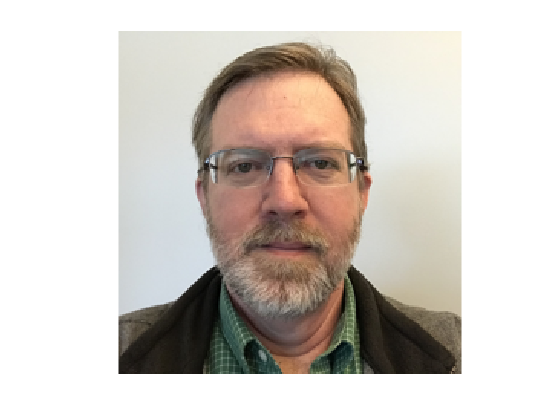
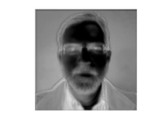
To experiment with this network, I'll use a picture that I took of myself just now. I will go ahead and resize it to the size expected by the network.
im = imread('steve.jpg');
im = imresize(im,net.Layers(1).InputSize(1:2));
imshow(im)
Use the
act = activations(net,im,'conv1-7x7_s2','OutputAs','channels');
size(act)
ans = 1×3

   112   112    64
I interpret the size of
min(act(:))
ans = single
    -2.9851e+03
max(act(:))
ans = single
    2.7232e+03
The functions
act = reshape(act,size(act,1),size(act,2),1,size(act,3));
act_scaled = mat2gray(act);
montage(act_scaled)
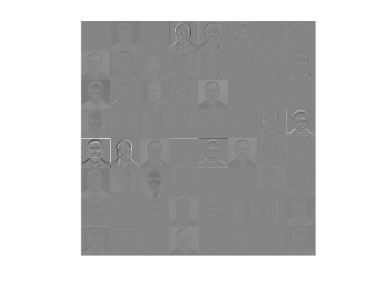
I think it will be easier to see and compare the individual activation images if we apply a contrast stretch. I'll use the Image Processing Toolbox functions
tmp = act_scaled(:);
tmp = imadjust(tmp,stretchlim(tmp));
act_stretched = reshape(tmp,size(act_scaled));
montage(act_stretched)
title('Activations from the conv1-7x7_s2 layer','Interpreter','none')

Wow. That's a little bit too much of me all at once. Let's zoom in on just a couple of the activation images.
subplot(1,2,1)
imshow(act_stretched(:,:,:,33))
title('Channel 33')
subplot(1,2,2)
imshow(act_stretched(:,:,:,34))
title('Channel 34')
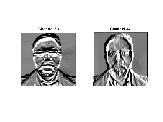
From my background in traditional image processing, I kind of recognize these. They are like gradient component images. One "detects" horizontal edges, and the other detects vertical edges.
We can see that if we look at the frequency responses of the weights for those layers.
w = net.Layers(2).Weights;
w33 = w(:,:,:,33);
clf
mesh(abs(freqz2(w33(:,:,2))),'EdgeColor',[0 .4470 .7410]);
title('Frequency response of the 33rd filter (green channel)')
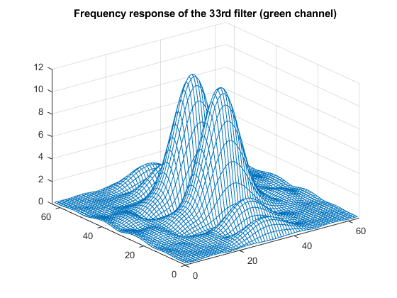
Roughly speaking, that's a bandpass filter in one direction and a lowpass filter in the other. In both directions, the filter cuts off most of the signal in the upper half of the frequency range, which is what I expect from an antialiasing filter designed for use with a factor-of-two downsampling.
w34 = w(:,:,:,34);
mesh(abs(freqz2(w34(:,:,2))),'EdgeColor',[0 .4470 .7410]);
title('Frequency response of the 34th filter (green channel)')
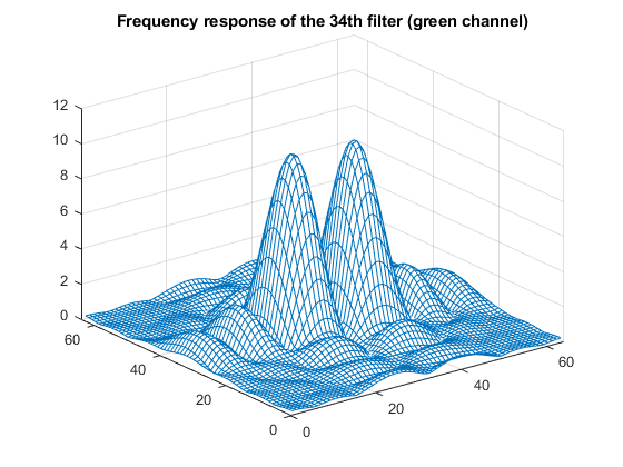
For this channel, the bandpass and lowpass directions are reversed.
I assume that these filter weights are derived from the training procedure used to create GoogLeNet in the first place. But it does seem like at least some parts of the network can be loosely interpreted in terms of traditional image processing operations.
Now let's look at the output of filter 43.
imshow(act_stretched(:,:,:,43))
I would guess that this filter output is serving a kind of color detection function. You can see a relatively high response for my green shirt, and a relatively low response for the skin tones in my face. Here are the weights for three channels of filter 43.
w43 = w(:,:,:,43);
subplot(2,2,1)
surf(w43(:,:,2),'EdgeColor',[0 .4470 .7410])
zlim([-0.3 0.3])
title('Green channel weights')
subplot(2,2,2)
surf(w43(:,:,1),'EdgeColor',[0 .4470 .7410])
zlim([-0.3 0.3])
title('Red channel weights')
subplot(2,2,3)
surf(w43(:,:,3),'EdgeColor',[0 .4470 .7410])
zlim([-0.3 0.3])
title('Blue channel weights')
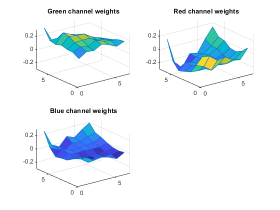
I don't quite have a good interpretation for everything I see here, but I have noticed that the inner portion of the weights for each channel looks fairly flat. Let me zoom in the x and y directions.
subplot(2,2,1)
xlim([3 5])
ylim([3 5])
subplot(2,2,2)
xlim([3 5])
ylim([3 5])
subplot(2,2,3)
xlim([3 5])
ylim([3 5])
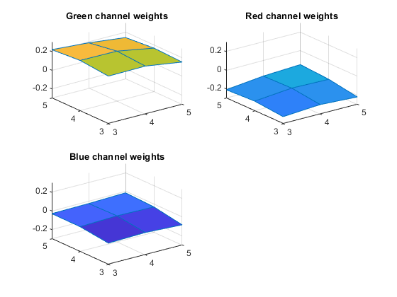
So, very roughly speaking, what's being computed is the difference between the local average of the green channel and the local average of the red channel.
Let's look at just one more layer, the one immediately following.
net.Layers(3)
ans =
  ReLULayer with properties:

    Name: 'conv1-relu_7x7'
This is a rectified linear unit layer. Such a layer just clips any negative number to 0. That means all the variation in the negative values from the output of the previous layer gets removed. What does that look like?
act2 = activations(net,im,'conv1-relu_7x7');
act2 = reshape(act2,size(act2,1),size(act2,2),1,size(act2,3));
act2_scaled = mat2gray(act2);
tmp = act2_scaled(:);
lim = stretchlim(tmp);
lim(1) = 0;
tmp = imadjust(tmp,lim);
act2_stretched = reshape(tmp,size(act2_scaled));
clf
montage(act2_stretched)
title('Activations from the conv1-relu_7x7 layer','Interpreter','none')
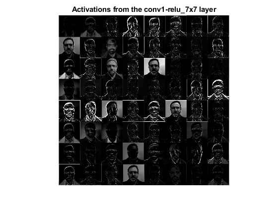
That's two layers down, and 142 still to go! I think I'll save those for another time.
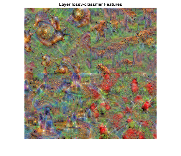
I encourage you to take a look at the documentation example Visualize Activations of a Convolutional Neural Network for another peek at the dreams of a deep learning neural network.
- Category:
- Deep Learning


Comments
To leave a comment, please click here to sign in to your MathWorks Account or create a new one.