| We have a very special post today from Jakob Kather from Heidelberg, Germany (Twitter: jnkath). He will be talking about deep learning for medical applications. Jakob is also one of the authors of a new paper recently published in Nature Medicine: https://www.nature.com/articles/s41591-019-0462-y discussing deep learning predicting gastrointestinal cancer. |
 |
Deep learning-based image analysis is well suited to classifying cats versus dogs, sad versus happy faces, and pizza versus hamburgers. However, many people struggle to apply deep learning to medical imaging data. In theory, it should be easy to classify tumor versus normal in medical images; in practice, this requires some tricks for data cleaning and model training and deployment.
Here, we will show how to use deep learning in MATLAB to preprocess and classify complex medical images. For this demo, we'll be primarily using Deep Learning Toolbox and Image Processing Toolbox. On the hardware side, it's best to have a compatible GPU installed and ready to use in MATLAB (see
https://www.mathworks.com/solutions/gpu-computing.html).
Our aim is to find tumor tissue in histological images**.
**Do you wonder what "histological images" are? In almost all cancer patients, the tumor is cut out by a surgeon, thinly sliced, put onto glass slides, stained and viewed under a microscope. Thus, we can see everything from cells on a micrometer scale to tissue structures on a millimeter scale.
Thousands of such images are freely available in public repositories. Some of these repositories are available at the National Institutes of Health (NIH) data portal. From
https://portal.gdc.cancer.gov we can download tumor images such as this (in this case, a lung cancer):

These images are in SVS format, which is essentially a multi-layer TIFF image.
This may look like an ordinary image, but SVS images are huge: the files are often larger than 1 GB and the images have up to a billion pixels. A zoomed in version of one section of this image shows how large this image is:
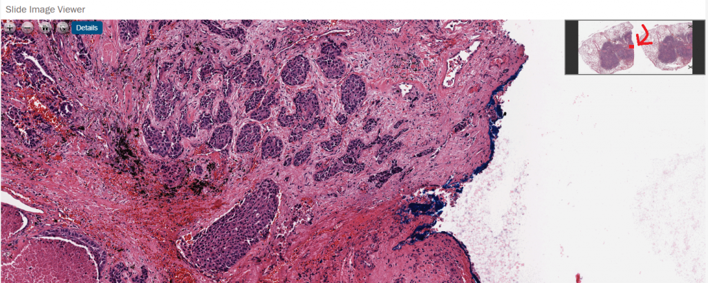
This image shows how much detail is contained in a very small portion of the image. We are zoomed in on the red dot shown in the upper right full image viewer.
Images courtesy of National Cancer Institute.
Many people struggle to even load these images, but MATLAB has some nice functions to deal with this huge amount of data. In particular, we will be using the functions imfinfo (to extract metadata), imread (to read the thumbnail) and blockproc (to read the actual image data without loading the full image into RAM).
So, let's use MATLAB to look at these images. We start by downloading an example image from the TCGA database. The image in this post can be found here:
https://portal.gdc.cancer.gov/files/0afb5489-719c-4e4d-bb8a-e0e146f0adb2
% define the image name
imName = 'TCGA-NK-A5CR-01Z-00-DX1.A7C57B30-E2C6-4A23-AE71-7E4D7714F8EA.svs';
imInfo = imfinfo(imName); % get the metadata
SVS images are essentially multipage TIFFs and we can use imfinfo() to look at the metadata of each page.
for i = 1:numel(imInfo)
    X = ['Layer ', num2str(i), ': Width ',num2str(imInfo(i).Width), ...
     ' and Height ', num2str(imInfo(i).Height)];
    disp(X)
end
The base image (channel 1) is so big that we cannot even look at it... but let's look at some of the smaller images instead.
imshow(imread(imName,2))
imshow(imread(imName,6))
imshow(imread(imName,7))
For each channel, we can look at the metadata.
disp(['this image has ',num2str(imInfo(5).Width),'*',num2str(imInfo(5).Height),' pixels'])
>> this image has 3019*1421 pixels
We can see this image is mostly background and contains non-tumor and tumor tissue. Because we care about the tumor tissue and not so much about the surrounding normal tissue, we want to identify the tumor region.
Note if you are a non-medical person, here is the image annotated with the tumor labeled.

Let us use a transfer learning approach with AlexNet. We will load the default pretrained AlexNet model which has already learned to distinguish shapes such as circles or lines.
net = alexnet; % load an alexnet which is pretrained on ImageNet
Now, we want to re-train the model as a tumor detector. We will use a public data set of 100,000 histological images of colon cancer, which is available at
http://dx.doi.org/10.5281/zenodo.1214456. This set has been derived from colorectal cancer samples, but the workflow is identical for any type of solid tumor.
This is how these smaller images (patches) look: They are labeled with one of nine classes which are explained in more detail in the data repository. Our aim is to train a deep neural network to automatically detect these classes.
 These images represent different classes of tissue that were manually defined by a pathologist. Each row is a tissue class and contains random images from the images set. The class labels are as follows: ADI = adipose tissue (fat), BACK = background (no tissue), DEB = debris, LYM = lymphocytes, MUC = mucus, MUS = muscle, NORM = normal mucosa, STR = stroma, TUM = tumor epithelium.The classes are described in more detail here: https://journals.plos.org/plosmedicine/article?id=10.1371/journal.pmed.1002730 and here: https://www.nature.com/articles/srep27988.
After downloading the ZIP files from the repository and extracting them to a folder called "images", we have one sub-folder per tissue class in "images." We can now load them, split into a training, validation and test set, and re-train our alexnet model. (Optionally, we could use the
imageDataAugmenter to create even more training images with rotational variance, for example).
Collect all pictures from the folder image and put them in a datastore. Subfolders are included, the category/label is determined by the folder names.
allImages = imageDatastore('./images/','IncludeSubfolders',true,'LabelSource','foldernames');
Split into three sets: 40% training, 20% validation, 40% test
[training_set, validation_set, testing_set] = splitEachLabel(allImages,.4,.2,.4);
Network modification
Modify the network by removing the last three layers. We will replace these layers with new layers for our custom classification.
layersTransfer = net.Layers(1:end-3);
Display the output categories.
categories(training_set.Labels)
ans =
9×1 cell array
| {'ADI'} |
| {'BACK'} |
| {'DEB'} |
| {'LYM'} |
| {'MUC'} |
| {'MUS'} |
| {'NORM'} |
| {'STR'} |
| {'TUM'} |
numClasses = numel(categories(training_set.Labels));
We merge the layers, and set the weight and bias learning rate for the last fully connected layer 'fc'
layers = [
    layersTransfer
    fullyConnectedLayer(numClasses,'Name', 'fc','WeightLearnRateFactor',1,'BiasLearnRateFactor',1)
    softmaxLayer('Name', 'softmax')
    classificationLayer('Name', 'classOutput')];
Set up a layerGraph and plot it:
lgraph = layerGraph(layers);
plot(lgraph)

Modify Training Parameters
We now modify the training set and training options. The training set must be resized to fit the input size expected by the network.
imageInputSize = [227 227 3];
augmented_training_set = augmentedImageSource(imageInputSize,training_set);
augmented_training_set =
augmentedImageDatastore with properties:
| NumObservations: 39999 |
| Files: {39999×1 cell} |
| AlternateFileSystemRoots: {} |
| MiniBatchSize: 128 |
| DataAugmentation: 'none' |
| ColorPreprocessing: 'none' |
| OutputSize: [227 227] |
| OutputSizeMode: 'resize' |
| DispatchInBackground: 0 |
resized_validation_set = augmentedImageDatastore(imageInputSize,validation_set);
resized_testing_set = augmentedImageDatastore(imageInputSize,testing_set);
Set the training options, including plotting the training progress as the network trains.
opts = trainingOptions('sgdm', ...
    'MiniBatchSize', 64,... % mini batch size, limited by GPU RAM, default 100 on Titan, 500 on P6000
    'InitialLearnRate', 1e-5,... % fixed learning rate
    'L2Regularization', 1e-4,... % optimization L2 constraint
    'MaxEpochs',15,... % max. epochs for training, default 3
    'ExecutionEnvironment', 'gpu',...% environment for training and classification, use a compatible GPU
    'ValidationData', resized_validation_set,...
    'Plots', 'training-progress')
Training
We trained the network for 3.5 hours on a single GPU, but training for a few minutes would actually be enough to get a reasonable result as seen in the training plot below.
net = trainNetwork(augmented_training_set, lgraph, opts)

Testing and Prediction
Let's check how well our classifier works using the held-out subset.
[predLabels,predScores] = classify(net, resized_testing_set, 'ExecutionEnvironment','gpu');
We can look at the confusion matrix and at the overall classification accuracy:
plotconfusion(testing_set.Labels, predLabels)
PerItemAccuracy = mean(predLabels == testing_set.Labels);
title(['overall per image accuracy ',num2str(round(100*PerItemAccuracy)),'%'])
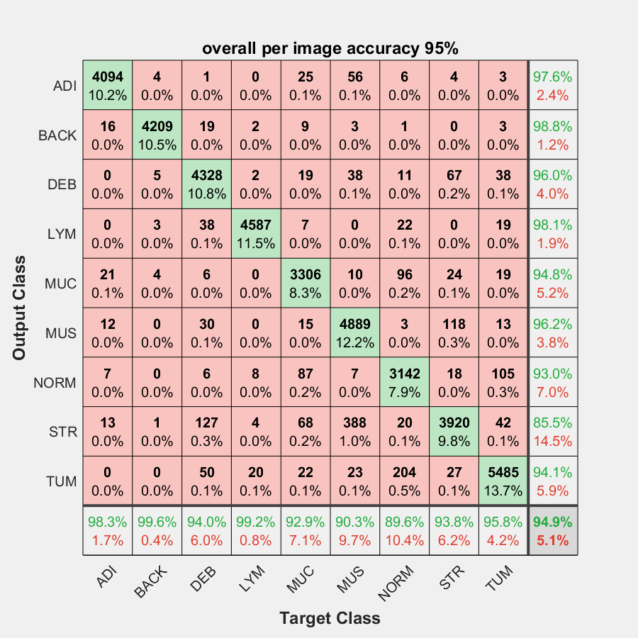
Voila! We have achieved an excellent classification performance (as you will see in
this paper). We are now ready to build more complicated workflows for digital pathology that include an automatic tumor detector!
I want to thank Jakob again for taking the time to give us insight into his research using MATLAB. A special thanks to Jakob Sommer for testing the source code in this post. Have any questions about this post? Leave a comment below.
 These images are in SVS format, which is essentially a multi-layer TIFF image.
This may look like an ordinary image, but SVS images are huge: the files are often larger than 1 GB and the images have up to a billion pixels. A zoomed in version of one section of this image shows how large this image is:

 Let us use a transfer learning approach with AlexNet. We will load the default pretrained AlexNet model which has already learned to distinguish shapes such as circles or lines.
 These images represent different classes of tissue that were manually defined by a pathologist. Each row is a tissue class and contains random images from the images set. The class labels are as follows: ADI = adipose tissue (fat), BACK = background (no tissue), DEB = debris, LYM = lymphocytes, MUC = mucus, MUS = muscle, NORM = normal mucosa, STR = stroma, TUM = tumor epithelium.The classes are described in more detail here: https://journals.plos.org/plosmedicine/article?id=10.1371/journal.pmed.1002730 and here: https://www.nature.com/articles/srep27988.
After downloading the ZIP files from the repository and extracting them to a folder called "images", we have one sub-folder per tissue class in "images." We can now load them, split into a training, validation and test set, and re-train our alexnet model. (Optionally, we could use the imageDataAugmenter to create even more training images with rotational variance, for example).
Collect all pictures from the folder image and put them in a datastore. Subfolders are included, the category/label is determined by the folder names.


 These images are in SVS format, which is essentially a multi-layer TIFF image.
This may look like an ordinary image, but SVS images are huge: the files are often larger than 1 GB and the images have up to a billion pixels. A zoomed in version of one section of this image shows how large this image is:

 Let us use a transfer learning approach with AlexNet. We will load the default pretrained AlexNet model which has already learned to distinguish shapes such as circles or lines.
 These images represent different classes of tissue that were manually defined by a pathologist. Each row is a tissue class and contains random images from the images set. The class labels are as follows: ADI = adipose tissue (fat), BACK = background (no tissue), DEB = debris, LYM = lymphocytes, MUC = mucus, MUS = muscle, NORM = normal mucosa, STR = stroma, TUM = tumor epithelium.The classes are described in more detail here: https://journals.plos.org/plosmedicine/article?id=10.1371/journal.pmed.1002730 and here: https://www.nature.com/articles/srep27988.
After downloading the ZIP files from the repository and extracting them to a folder called "images", we have one sub-folder per tissue class in "images." We can now load them, split into a training, validation and test set, and re-train our alexnet model. (Optionally, we could use the imageDataAugmenter to create even more training images with rotational variance, for example).
Collect all pictures from the folder image and put them in a datastore. Subfolders are included, the category/label is determined by the folder names.




Comments
To leave a comment, please click here to sign in to your MathWorks Account or create a new one.