
Advanced Deep Learning: Part 1
Build any Deep Learning Network
For the next few posts, I would like us all to step out of our comfort zone. I will be exploring and featuring more advanced deep learning topics. Release 19b introduced many new and exciting features that I have been hesitant to try because people start throwing around terms like, custom training loops, automatic differentiation (or even “autodiff” if you’re really in the know). But I think it’s time to dive in and explore new concepts, not just to understand them but understand where and why to use them.
There is a lot to digest beyond the basics of deep learning, so I’ve decided to create a series of posts. The post you are reading now will serve as a gentle introduction to lay groundwork and key terms, followed by a series of posts that look at individual network types (Autoencoders, Siamese networks, GANs and Attention mechanisms).
The advanced deep learning basics
First, let’s start with the why: "why should I bother using the extended deep learning framework? I've gotten by just fine until now." First, you get a flexible training structure which allows you to create any network in MATLAB. The more complicated structures featured in the next posts require the extended framework to address features like:
 A dlnetwork has properties such as layers and connections (which can handle Series or DAG networks) and also a place to store 'Learnables'. More on this later.
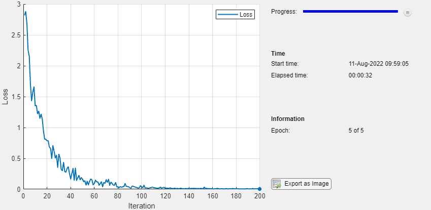
 You'll notice quite a few more non-optional parameters explicitly defined: these are parameters you will use in the custom training loop. Also, we no longer have the option of a pretty training plot like in the basic framework.
 Basics you need to know before going into the training loop:
 So according to our defined parameters above, our custom training loop will loop through the entire dataset 30 times, and since our mini-batch size is 128, and our total number of images is 5000, it'll take 39 iterations to loop through the data 1 time.
Here's the structure of the custom training loop. The full code is in the doc example, and I'll warn you the full script is quite a few lines of code, but a lot of it is straightforward once you understand the overall structure.
So according to our defined parameters above, our custom training loop will loop through the entire dataset 30 times, and since our mini-batch size is 128, and our total number of images is 5000, it'll take 39 iterations to loop through the data 1 time.
Here's the structure of the custom training loop. The full code is in the doc example, and I'll warn you the full script is quite a few lines of code, but a lot of it is straightforward once you understand the overall structure.
 And as you may have guessed based on what's highlighted in the visualization above, the next post in this series will go into more detail on the inner workings of the loop, and what you need to know to understand what's happening with loss, gradients, learning rate, and updating network parameters.
Three model approaches
One final point to keep in mind, while I used the extended framework with the DLNetwork approach, there is also a Model Function approach to use when you also want control of initializing and explicitly defining the network weights and biases. The example can also use the model function approach and you can follow along with this doc example to learn more. This approach gives you the most control of the 3 approaches, but is also the most complex.
The entire landscape looks like this:
And as you may have guessed based on what's highlighted in the visualization above, the next post in this series will go into more detail on the inner workings of the loop, and what you need to know to understand what's happening with loss, gradients, learning rate, and updating network parameters.
Three model approaches
One final point to keep in mind, while I used the extended framework with the DLNetwork approach, there is also a Model Function approach to use when you also want control of initializing and explicitly defining the network weights and biases. The example can also use the model function approach and you can follow along with this doc example to learn more. This approach gives you the most control of the 3 approaches, but is also the most complex.
The entire landscape looks like this:
 That's it for this post. It was a lot of information, but hopefully you found something informative within it. If you have any questions or clarifications, please leave a comment below!
- Multiple Inputs and Outputs
- Custom loss functions
- Weight sharing
- Automatic Differentiation
- Special visualizations during training
- Define Network Layers
- Specify Training Options
- Train Network
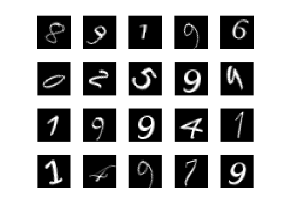
Load the data
[XTrain,YTrain] = digitTrain4DArrayData;
[XTest, YTest] = digitTest4DArrayData;
classes = categories(YTrain);
numClasses = numel(classes);
1. Define Network Layers
Create a network, consisting of a simple series of layers.layers = [
imageInputLayer([28 28 1])
convolution2dLayer(5,20,'Padding','same')
batchNormalizationLayer
reluLayer
maxPooling2dLayer(2,'Stride',2)
fullyConnectedLayer(10)
softmaxLayer
classificationLayer];
2. Specify Training Options
options = trainingOptions('sgdm', ...
    'InitialLearnRate',0.01, ...
    'MaxEpochs',4, ...
    'Plots','training-progress');
These are simple training options, and not necessarily intended to give the best results. In fact, trainingOptions only requires you to set the optimizer, and the rest can use default values.
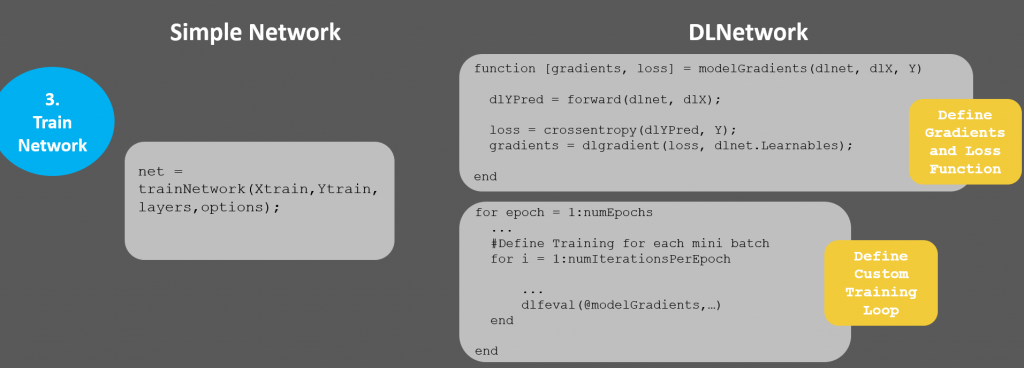
3. Train the network
net = trainNetwork(XTrain,YTrain,layers,options);Simple enough! Now let's do the same thing in the extended framework. Extended Framework Example Same example, just using the extended framework, or "DLNetwork" as I'll refer to this approach moving forward. This is a modified version of the code. To follow along with the complete example, the full code is in the doc example.
Load data
This is exactly the same, no need to show repeat code. Now we can show the differences between the simple approach and the DLNetwork approach: Let's compare each of the following steps side by side to see highlight the differences.
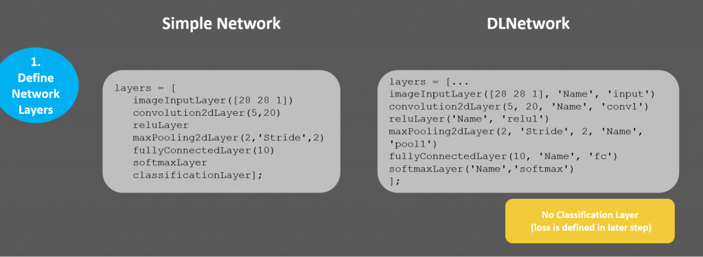
1. Define Network Layers
Layers are almost the same: we just need add names for each of the layers. This is handled explicitly in the simple framework, but we're required to do a little more pre-work.layers = [...
imageInputLayer([28 28 1], 'Name', 'input','Mean',mean(Xtrain,4))
convolution2dLayer(5, 20, 'Name', 'conv1')
reluLayer('Name', 'relu1')
maxPooling2dLayer(2, 'Stride', 2, 'Name', 'pool1')
fullyConnectedLayer(10, 'Name', 'fc')
softmaxLayer('Name','softmax')
];
Notice in the layers, there is no classification layer anymore. This will be handled in the training loop, since this is what we want to customize.
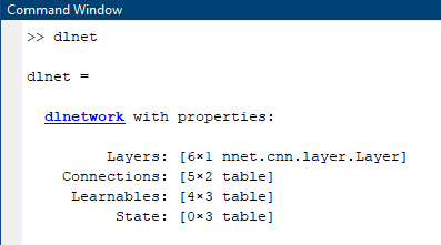
Then convert the layers into a layerGraph, which makes them usable in a custom training loop. Also, specify the dlnet structure containing the network.
lgraph = layerGraph(layers);
dlnet = dlnetwork(lgraph);
A dlnetwork has properties such as layers and connections (which can handle Series or DAG networks) and also a place to store 'Learnables'. More on this later.
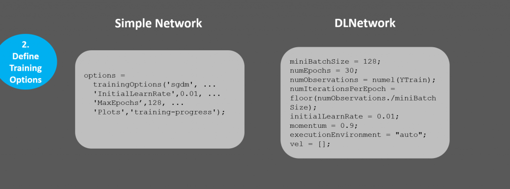
2. Specify Training Options
 You'll notice quite a few more non-optional parameters explicitly defined: these are parameters you will use in the custom training loop. Also, we no longer have the option of a pretty training plot like in the basic framework.
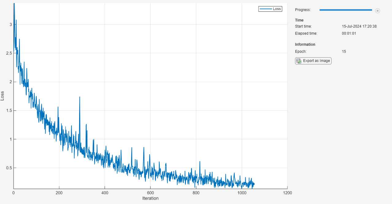
miniBatchSize = 128;
numEpochs = 30;
numObservations = numel(YTrain);
numIterationsPerEpoch = floor(numObservations./miniBatchSize);
initialLearnRate = 0.01;
momentum = 0.9;
executionEnvironment = "auto";
vel = [];
You are now responsible for your own visualization, but this also means you could create your own visualizations throughout training, and customize to your liking to show anything about the network that would help to understand the network as it trains. For now, let's setup a plot to display the loss/error as the network trains.
plots = "training-progress";
if plots == "training-progress"
    figure
    lineLossTrain = animatedline;
    xlabel("Total Iterations")
    ylabel("Loss")
end
Train network using custom training loop
 Basics you need to know before going into the training loop:
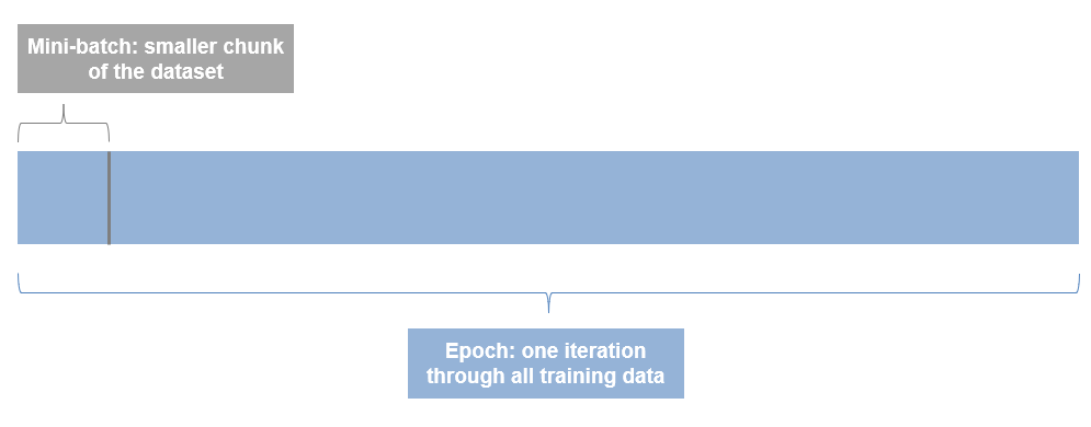
- An Epoch is one iteration through the entire dataset. So if you have 10 epochs, you are running through all files 10 times.
- A Mini-batch is a smaller chunk of the dataset. Datasets are often too big to fit in memory or on a GPU at the same time, so we process the data in batches.
So according to our defined parameters above, our custom training loop will loop through the entire dataset 30 times, and since our mini-batch size is 128, and our total number of images is 5000, it'll take 39 iterations to loop through the data 1 time.
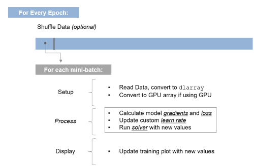
Here's the structure of the custom training loop. The full code is in the doc example, and I'll warn you the full script is quite a few lines of code, but a lot of it is straightforward once you understand the overall structure.
for epoch = 1:numEpochs
     ...
  for ii = 1:numIterationsPerEpoch
    % *Setup: read data, convert to dlarray, pass to GPU
           ...

    % Evaluate the model gradients and loss
    [gradients, loss] = dlfeval(@modelGradients, dlnet, dlX, Y);

    % Update custom learn rate
    learnRate = initialLearnRate/(1 + decay*iteration);

    % Update network parameters using SGDM optimizer
    [dlnet.Learnables, vel] = sgdmupdate(dlnet.Learnables, gradients, vel, learnRate, momentum);

    % Update training plot
        ...
  end
end
For completeness, you create the function modelGradients where you define the gradients and loss function. More on the specifics of this in the next post.
function [gradients, loss] = modelGradients(dlnet, dlX, Y)

  dlYPred = forward(dlnet, dlX);

  loss = crossentropy(dlYPred, Y);
  gradients = dlgradient(loss, dlnet.Learnables);

end
In the simple example, one function trainnetwork has expanded into a series of loops and code. We're doing this so we have more flexibility when networks require it, and we can revert back to the simpler method when it's overkill. The good news is, this is as complicated as it gets: Once you understand this structure, it's all about putting the right information into it! For those that want to visualize what's happening in the loop, I see it like this:
And as you may have guessed based on what's highlighted in the visualization above, the next post in this series will go into more detail on the inner workings of the loop, and what you need to know to understand what's happening with loss, gradients, learning rate, and updating network parameters.
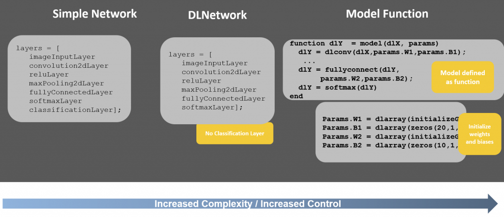
Three model approaches
One final point to keep in mind, while I used the extended framework with the DLNetwork approach, there is also a Model Function approach to use when you also want control of initializing and explicitly defining the network weights and biases. The example can also use the model function approach and you can follow along with this doc example to learn more. This approach gives you the most control of the 3 approaches, but is also the most complex.
The entire landscape looks like this:
 That's it for this post. It was a lot of information, but hopefully you found something informative within it. If you have any questions or clarifications, please leave a comment below!
- 범주:
- Deep Learning


댓글
댓글을 남기려면 링크 를 클릭하여 MathWorks 계정에 로그인하거나 계정을 새로 만드십시오.