
Optimization of HRTF Models with Deep Learning
Today’s post is from Sunil Bharitkar, who leads audio/speech research in the Artificial Intelligence & Emerging Compute Lab (AIECL) within HP Labs. He will discuss his research using deep learning to model and synthesize head-related transfer functions (HRTF) using MATLAB. This work has been published in an IEEE paper, linked at the bottom of the post.
Today I’d like to discuss my research, which focuses on a new way to model how to synthesize sound from any direction at all angles using deep learning.
If we look at this plot, you can see that when a sound is played at a direction of 45 degrees from the center, the sound at the left ear is higher in amplitude at this angle than the right. Also embedded in this plot is the difference in arrival time between the left and right ear, where only a few milliseconds in difference can have an important impact on where we perceive sound. Subconsciously, we interpret the location of the sound source based on this difference in spectra and delay.
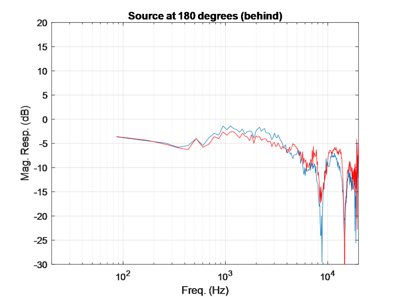
Compare this with a sound coming 180 degrees behind a human:
The spectral detail at the left and right ear is nearly identical at all frequencies, since the sound source is substantially equidistant from both ears. The difference in arrival time will be insignificant for the sounds source at 180 degrees. These discrepancies (or lack thereof) is what helps us determine where sounds is coming from.
We are very good at localizing sound at certain frequencies, and not as good at others*. This depends on the frequency and the location of the sound.
*It’s interesting to note that humans aren’t very good at determining whether sound in certain angles (e.g., in the cone of confusion). The best way we can help to localize if we are confused is to move our head around to try to optimize the discrepancies between left and right ear. I’m sure you’re now curious to try this experiment informally at home with your next beeping fire alarm.
This research has many applications where localization of sound is critical. One example is in video game design, or virtual reality, where the sound must match the video for a truly immersive experience. For sound to match video, we must match the expected cues for both ears at desired locations around the user.
There are many aspects of this research which makes this a challenging problem to solve:
Our anatomies and our hearing are a unique quality each human has for themselves. The only way to be 100% confident the sound will be perfect for a person will be to measure their individualized head related transfer function in an anechoic chamber. This is highly impractical, as our goal is to have the least setup time for the consumer. So this leads us to the main aspect of my research:
Can we use deep learning to approximate an HRTF at all angles for a genuine experience for a large number of listeners?
This formula says, for a given user at a given angle and certain frequency bin, compare the actual amplitude vs. the network’s given response.
For PCA, we found that 10 PCs was a fair comparison to our model (as shown in the figure below), since this allowed for the most of this large dataset to be covered properly by this method.
 Here’s a random sampling for test subjects, for given angles, showing the results between the AE approach vs. the PCA. You can see for the most part, you can see significant improvements using the deep learning approach.
 Another nice visualization I created clearly shows the difference between models:
The two models are compared using log-spectral distortion (dLS) for each angle and each user. A green box is an indication the dLS is lower than the PCA (lower is better). And the blue is where the PCA based approach outperforms the autoencoder. As you can see, for the most part, the AE encoder outperforms the PCA. The AE approach is not 100% better, but certainly a much better result overall.
In conclusion, we showed a new deep learning approach showing significant improvement representing a large subject-pool HRTFs over the state-of-the-art PCA approach. We are continuing to test on much larger datasets, and we are continuing to see reproducible results even over larger dataset sizes, so we are confident this approach is producing consistent results.
If you would like to learn more on this topic, the link to the entire paper, which received the Outstanding Paper Award from the IEEE is here https://ieeexplore.ieee.org/document/8966196.
A crash course in Spatial Audio
One important aspect of this research is in the localization of sound. This is studied quite broadly for audio applications and relates to how we as humans hear and understand where sound is coming from. This will vary person to person, but it generally has to do with the delay relative to each ear (below ~800 Hz) and spectral details at the individual ears at frequencies greater than ~ 800 Hz. These are primarily the cues that we use to localize sound on a daily basis (for example see the cocktail party effect). Below are figures displaying the Head-Related impulse response measured in an anechoic chamber at the entrance of both ear-canals of a human subject (left figure), and the Fourier-domain representation i.e., the Head-related Transfer function (right figure), which shows how a human hears sound at both ears at a certain location (e.g., 45 degrees to the left and front and 0 degrees elevation) in the audible frequencies. |
 |
- Humans are very good at spotting discrepancies in sound, which will appear fake and lead to a less than genuine experience for the user.
- Head related transfer functions are different for different people over all angles.
- Each HRTF is direction dependent and will vary at each angle for any given person.

Current state of the art vs. our new approach
The question you might be asking is “well, if everyone is different, why not just take the average of all the plots and create an average HRTF?” To that, I say “if you take the average, you’ll just have an average result.” Can deep learning help us improve on the average? Prior to our research, the primary method to perform this analysis was principle component analysis for HRTF modeling over a set of people. In the past, researchers have found 5 or 6 components used that generalize as well as they can for a small test set of approximately 20 subjects([1] [2] [3]) but we want to generalize over a larger dataset and a larger number of angles. We are going to show a new approach using deep learning. We are going to apply this to an autoencoder approach for learning a lower dimensional representation (latent representation) of HRTFs using nonlinear functions, and then using another network (a Generalized Regression neural network in this case) to map angles to the latent representation. We start with an autoencoder of 1 hidden layer, and then we optimize the number of hidden layers and the spread of the Gaussian RBF in the GRNN by doing Bayesian optimization with a validation metric (the log-spectral distortion metric). The next section shows the details of this new approach.New approach
For our approach we are using the IRCAM dataset, which consists of 49 subjects with 115 directions of sound per subject. We are going to use an autoencoder model and compare this against the principle component analysis model, (which is a linearly optimal solution conditioned on the number of PC’s) and we will compare the results using objective comparisons using log spectral distortion metric to compare performance.Data setup
As I mentioned, the dataset has 49 subjects, 115 angles and each HRTF is created by computing the FFT over 1024 frequency bins. Problem statement: can we find an HRTF representation for each angle that best maximizes the fit over all subjects for that angle? We’re essentially looking for the best possible generalization, over all subjects, for each of the 115 angles.- We also used hyperparameter tuning (bayesopt) for the deep learning model.
- We take the entire HRTF dataset (1024X5635) and train the autoencoder. The output of the hidden layer gives you a compact representation of the input data. We take the autoencoder, we extract that representation and then map that back to the angles using a Generalized RNN. We also add jitter, or noise that we add for each angle and for each subject. This will help the network generalize rather than overfit, since we aren’t looking for the perfect answer (this doesn’t exist!) rather the generalization that best fits all test subjects.
- Bayesian optimization was used for:
- The size of the autoencoder network (the number of layers)
- The jitter/noise variance added to each angle
- The RBF spread for the GRNN
Results
We optimized the Log-spectral distortion to determine the results:
Selection of PCA-order (abscissa: no. of PC, ordinate: explained variance), (a) left-ear (b) right ear)
Example of the left-ear HRTF reconstruction comparison using AE-model (green) compared to true HRTF (blue). The PCA model is used as an anchor and is shown in red.

References
[1] D. Kistler, and F. Wightman, “A model of head-related transfer functions based on principal components analysis and minimum-phase reconstruction,” J. Acoust. Soc. Amer., vol. 91(3), 1992, pp. 1637-1647. [2] W. Martens, “Principal components analysis and resynthesis of spectral cues to perceived direction,” Proc. Intl. Comp. Mus. Conf., 1987, pp. 274-281. [3] J. Sodnik, A. Umek, R. Susnik, G. Bobojevic, and S. Tomazic, “Representation of Head-related Transfer Functions with Principal Component Analysis,” Acoustics, Nov. 2004.- Category:
- Deep Learning


Comments
To leave a comment, please click here to sign in to your MathWorks Account or create a new one.