Using Deep Learning for Complex Physical Processes
Guest Blog by: Peetak Mitra, Dr. Majid Haghshenas and Prof. David P. Schmidt
The following is an accepted paper at the Neural Information Processing Systems (NeurIPS) Machine Learning for Engineering Design, Simulation Workshop 2020. This work is a part of the ICEnet Consortium, an industry-funded effort in building data-driven tools relevant to modeling Internal Combustion Engines. More details can be found at icenetcfd.com
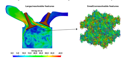
In recent years, there has been a surge of interest in using machine learning for modeling physics applications. Prof. Schmidt’s research group at UMass Amherst has been working towards applying these methods for turbulence closure, coarse-graining, combustion or building cheap-to-investigate emulators for complex physical process. In this blog, we will introduce the current challenges in applying mainstream machine learning algorithms to domains specific applications and will showcase how we dealt with this challenge in our scientific application of interest that is the closure modeling relevant to fluid turbulence.
Current Challenges
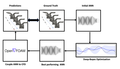
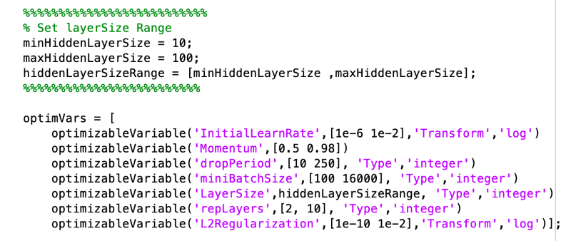
The ML algorithms and the best practices in designing the network and choosing hyperparameters therein, have been developed for applications such as computer vision, natural language processing among others. The loss manifold of these datasets is by nature vastly different than the one observed in the scientific datasets [see Figure 1 for an example, loss generated using a function of two variables, obtained by translating and scaling Gaussian distributions, a common distribution in science and engineering]. Therefore, often times these best practices from literature translate poorly to applications within scientific domain. Some major challenges in doing so include that the data used to develop machine learning algorithms differ from scientific data in fundamental ways; as the scientific data is often high-dimensional, multimodal, complex, structured and/or sparse [1]. The current pace of innovation in SciML is additionally driven by and limited to, the empirical exploration/experimentation with these canonical ML/DL techniques. In order to fully leverage the complicated nature of the data as well as develop optimized ML models, automatic machine learning (AutoML) methods for automating network design and choosing the best performing hyperparameters is critically required. In this work, we explore the effectiveness of Bayesian based AutoML methods for complex physics emulators in an effort to build robust neural network models.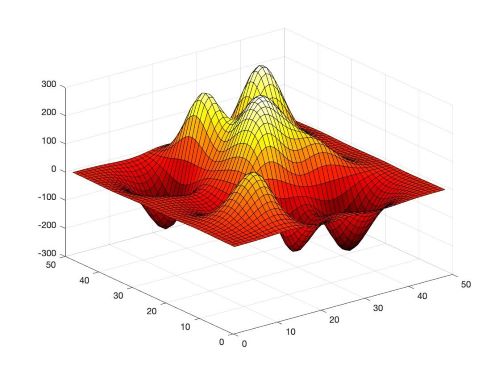


Results
We find that the ADAM Glorot and ADAM He combinations perform the best in terms of absolute errors, although the ADAM Glorot configuration has the highest number of parameters. The RMPSProp on average, performs better than SGDM optimizer. This can be explained as RMSProp is an adaptive learning rate method and is capable in navigating regions of local optima and whereas that SGDM performs poorly navigating ravines and makes hesitant progress towards local optima. The a-priori performance of the best performing model is shown in Figure 4.
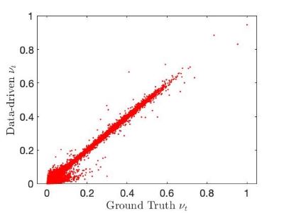
 Fig 5. Evolution of the learning process can be visualized using the cosine similarity during the network training checkpointed at every epoch.
 |
 |
Fig 6. Low-dimensional representation of the function-space similarity for the weight initialization and optimizers reveal important takeaways.
In summary, an AutoML in the training loop, provides a pathway to not only build robust neural networks suitable for applications to scientific datasets, but can be used to better understand the network training evolution process. To learn more about our work please follow the pre-print here, and watch the NeurIPS 2020 ML4Eng workshop spotlight talk here.References
[1]: Dias Ribeiro, Mateus, Alex Mendonça Bimbato, Maurício Araújo Zanardi, José Antônio Perrella Balestieri, and David P. Schmidt. "Large-eddy simulation of the flow in a direct injection spark ignition engine using an open-source framework." International Journal of Engine Research (2020): 1468087420903622- Category:
- Deep Learning




Comments
To leave a comment, please click here to sign in to your MathWorks Account or create a new one.