
Finding Information in a Sea of Noise
For today's blog, I would like to pose a problem:
Suppose that you had a lot of data representing something very random, but that had a very small "tell" that differentiated the data into two different classes--a single nucleotide defect in a noisy genome population, for instance. (Okay, maybe that's a stretch.) But given a single informative "bit" in a noisy dataset, how would you find that tell?
Contents
Let's create (and visualize) a dataset that sets up the question
First, create 10,000 random 20 x 20 matrices.
rng(0);
n = 10000;
sz = [20 20];
a = rand(sz(1), sz(2), 1, n);
Create a "Tell":
Now we will convert 1 randomly selected pixel to be modified as a class1/class2 "tell," or "indicator":
randomInformationalElement = randi(sz(1) * sz(2))
[rowIndTrue, colIndTrue] = ind2sub(size(a), randomInformationalElement);

% At that randomly selected location, we will set half of the images to
% have one random value, and the other half to have a different random
% value:

%Class 1:
class1Val = rand(1);
for ii = 1:n/2
 a(rowIndTrue, colIndTrue, ii) = class1Val;%1
end

%Class 2:
class2Val = rand(1);
for ii = n/2 + 1:n
 a(rowIndTrue, colIndTrue, ii) = class2Val;%0.5
end

% And we will create categorical labels to keep track of the "Class":
labels = [repmat(categorical("class1"), n/2, 1);
 repmat(categorical("class2"), n/2, 1)];
summary(labels)
randomInformationalElement =
   193
     class1      5000
     class2      5000
Let's take a look at three of each class...can you spot the tell?
figure('Name', 'Samples');
inds = [1:3, n-2:n];
layout = tiledlayout(2, 3, 'TileSpacing', 'compact');
ax = gobjects(2, 3);
ind = 1;
for ii = inds
 ax(ind) = nexttile(layout);
 imshow(a(:, :, ii))
 hold on
 if ind == 2
 title('CLASS 1', 'color', 'r', 'fontsize', 18);
 elseif ind == 5
 title('CLASS 2', 'color', 'r', 'fontsize', 18);
 end
 ind = ind + 1;
end

How about now?
for ii = 1:6
 plot(ax(ii), colIndTrue, rowIndTrue, 'gs', 'MarkerSize', 12, 'LineWidth', 2)
end
linkaxes(ax)
set(ax, 'xlim', [0.85*colIndTrue, 1.15*colIndTrue], ...
    'ylim', [0.85*rowIndTrue, 1.15*rowIndTrue])
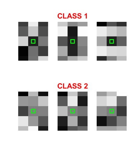
Where is the tell?
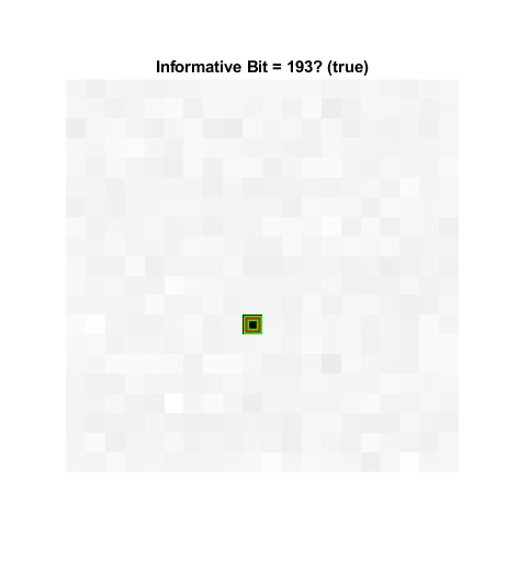
The goal here is to find a model to detect the informative bit--thereby separating the matrices into two classes. The perceptive reader might realize that one could simply look at the minimum standard deviation of the matrices, for example, to find the informative bit:
figure('Name', 'Found It!')
stdA = std(a, 1, ndims(a));
imshow(stdA, []);
title('Standard Deviation')
detection = find(stdA == min(stdA(:)));
[rowIndDetected, colIndDetected] = ind2sub(size(a), detection);
hold on
plot(colIndTrue, rowIndTrue, 'gs', 'MarkerSize', 12, 'LineWidth', 4)
plot(colIndDetected, rowIndDetected, 'rs', 'MarkerSize', 12, ...
    'LineWidth', 1.5);
if detection == randomInformationalElement
    detected = "true";
else
    detected = "false";
end
title("Informative Bit = " + detection + "? (" + detected + ")")
Obfuscating
So clearly this is a bit contrived. We could further obfuscate it by changing some values in confounding ways. For instance:
for jj = 1:10
    confounder = randi(sz(1) * sz(2));
    [rowInd, colInd] = ind2sub(size(a), confounder);
    R = rand(1);
    for ii = 1:2:n
        a(rowInd, colInd, ii) = R;
    end
    R = rand(1);
    for ii = 2:2:n
        a(rowInd, colInd, ii) = R;
    end
end

figure('Name', 'Obfuscated')
stdA = std(a, 1, ndims(a));
imshow(stdA, []);
title('Standard Deviation')
detection = find(stdA == min(stdA(:)));
[rowIndDetected, colIndDetected] = ind2sub(size(a), detection);
hold on
plot(colIndTrue, rowIndTrue, 'gs', 'MarkerSize', 12, 'LineWidth', 4)
plot(colIndDetected, rowIndDetected, 'rs', 'MarkerSize', 12, ...
    'LineWidth', 1.5);
if detection == randomInformationalElement
    detected = "true";
else
    detected = "false";
end
title("Informative Bit = " + detection + "? (" + detected + ")")
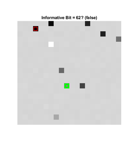
Now the information is more obscure!
A challenge:
Try to find this informative bit using "classical machine learning" (CML) models, leveraging tools like the classificationLearner App. In my experience, the models afforded by the classificationLearner will churn for a very long time (hours, even!), and none of the models will converge to anything better than 50%. That is, the models will be 100% useless! (I leave that trial to the reader. But I'll send a MATLAB T-shirt to the first person who shares with me a model trained with that app that reliably solves this problem!)
Constraints!
Why do CML models fail? In a word: constraints! Typically, to create an image classifier, we might first aggregate features using a "bag of features". Then, using those aggregated features, we could train an "image category classifier." (The trainImageCategoryClassifier function makes trivial work of that.) Note that using bagOfFeatures implicitly calculates SURF Features, and that trainImageCategoryClassifier implicitly trains a multiclass Support Vector Machine (SVM). Features characterize relationships between pixels, and it's not clear that either SURF or SVM are appropriate for the task at hand. And even if you used non-default detectors, extractors, and classifiers, you would still have a constrained model!
Enter Deep Learning
Deep learning is, in contrast, relatively unconstrained; we don't have to tell the model what relationships to look at. Rather, we can specify a "network architecture" and provide a bunch of "ground truth," and let the computer figure out what to look for!
For instance, here we create just about the simplest "typical" network architecture for classifying images:
sizeOfKernel = [5, 5];
numberOfFilters = 20;
nClasses = 2;
layers = [
 imageInputLayer([sz(1) sz(2) 1])
 convolution2dLayer(sizeOfKernel, numberOfFilters, 'Name', 'conv')
 reluLayer
 maxPooling2dLayer(2, 'Stride', 2)
 fullyConnectedLayer(nClasses, 'Name', 'fc')
 softmaxLayer
 classificationLayer()
 ];
That "triad" of "convolution, relu, and pooling" layers is very common in deep learning networks designed for image analysis. But note that we haven't overly constrained the model to consider only a specific feature- or model-type; we've simply told the model to calculate 20 5x5 convolutions. And more to the point, we haven't even specified what patterns (convolution kernels) to look for.
So let's create validation and test sets, and train the model
Creating a validation set will help us ensure that the model is not overfitting, and a test set will help us to evaluate the model after training.
% First, the validation set:
inds = 1:100:size(a, 4);
validationData = a(:, :, :, inds);
validationLabels = labels(inds);
% Remove the validation labels from the training set:
a(:, :, :, inds) = [];
labels(inds) = [];
% Now the test set:
inds = 1:100:size(a, 4);
testSet = a(:, :, :, inds);
testLabels = labels(inds);
a(:, :, :, inds) = [];
labels(inds) = [];

% ...Specify some training options:

miniBatchSize = 100;
options = trainingOptions( 'adam', ...
 'InitialLearnRate', 0.005, ...
 'MaxEpochs', 1000, ...
 'MiniBatchSize', miniBatchSize, ...
 'Plots', 'training-progress', ...
 'ValidationData', {validationData, validationLabels}, ...
 'ValidationFrequency', 10, ...
 'ValidationPatience', 30, ...
 'OutputFcn', @(info)stopIfAccuracyNotImproving(info, 50));

% ... and Train!
net = trainNetwork(a, labels, layers, options);
Training on single GPU.
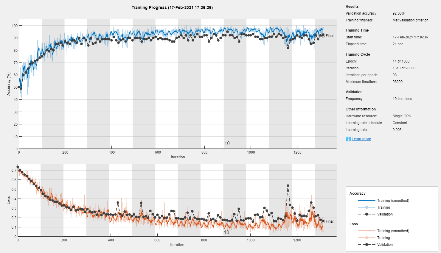
Wow...
In just under half a minute, this simple "deep" learning model appears to have converged to 95% accuracy!
predictedLabels = net.classify(testSet);
ind = randi(size(testSet, ndims(a)));
net.classify(testSet(:, :, :, ind));
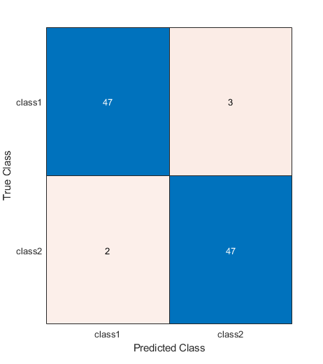
togglefig('Confusion Matrix')
m = confusionchart(testLabels, predictedLabels);
testAccuracy = sum(predictedLabels == testLabels) / numel(testLabels)
testAccuracy =
      0.94949
What's going on?
That's useful, but it's also puzzling: if the model has figured out where the "tell" is (which it must have done, or it couldn't have gotten above 50%), why then isn't it 100% accurate?
The answer to that lies in the network architecture. The "triad" of typical convolutional neural network (CNN) layers that we used includes a pooling layer. Since our information is a single bit, the pooling is "smearing" the information! What if we removed that layer?
layers = [
 imageInputLayer([sz(1) sz(2) 1])
 convolution2dLayer(sizeOfKernel, numberOfFilters, 'Name', 'conv')
 reluLayer
 fullyConnectedLayer(2, 'Name', 'fc')
 softmaxLayer
 classificationLayer()
 ];
net = trainNetwork(a, labels, layers, options);
predictedLabels = net.classify(testSet);
testAccuracy = sum(predictedLabels == testLabels) / numel(testLabels)
Training on single GPU.
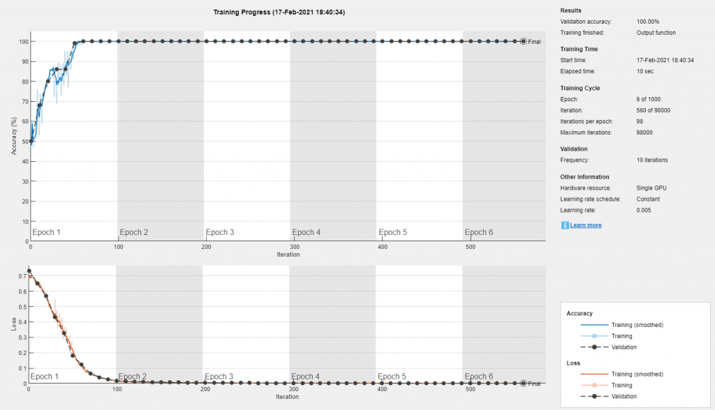
Sweet!
About 10 seconds to 100% accuracy! That helps us to understand what some of the layers are doing, and why we need to tailor the network to the task at hand! (Note that we could also remove the relu layer; it neither helps nor hinders the model in this particular case.)
Great! But can we determine the location of the tell?
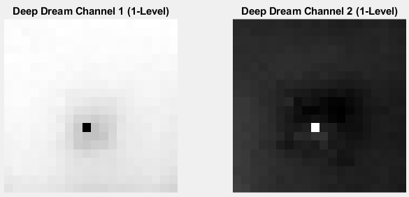
Yes! "Deep Dream" is your friend!
channels = [1, 2];
layer = 4; %Fully Connected
I = deepDreamImage(net, layer, channels, 'PyramidLevels', 1);
togglefig('Deep Dream');
subplot(1, 2, 1)
channel1Image = I(:, :, :, 1);
imshow(channel1Image);
title('Deep Dream Channel 1 (1-Level)')
subplot(1, 2, 2)
channel2Image = I(:, :, :, 2);
imshow(channel2Image);
title('Deep Dream Channel 2 (1-Level)')
[rmax, cmax] = find(channel1Image == min(channel1Image(:)));
% Or [rmax, cmax] = find(channel2Image == max(channel2Image(:)));
fprintf('TARGET:\t\tRowInd = %i;\tColInd = %i;\nDETECTION:\tRow = %i;\t\tCol = %i\n', rowIndTrue, colIndTrue, rmax, cmax)
|==============================================|
|  Iteration  |  Activation  |  Pyramid Level  |
|             |   Strength   |                 |
|==============================================|
|           1 |         1.55 |               1 |
|           2 |       265.54 |               1 |
|           3 |       533.66 |               1 |
|           4 |       804.17 |               1 |
|           5 |      1075.66 |               1 |
|           6 |      1347.60 |               1 |
|           7 |      1619.17 |               1 |
|           8 |      1891.03 |               1 |
|           9 |      2163.16 |               1 |
|          10 |      2435.12 |               1 |
|==============================================|
TARGET:		RowInd = 13;	ColInd = 10;
DETECTION:	Row = 13;		Col = 10
A final comment
When we talk about deep learning, "deep" refers typically to the number of layers in the network architecture. This model isn't really deep in that regard. But we did implement end-to-end learning (i.e., learning directly from data)--and that is another hallmark of deep learning.
I hope you found this interesting, even if it is a bit contrived. Your comments are welcome!
- Category:
- Deep Learning


Comments
To leave a comment, please click here to sign in to your MathWorks Account or create a new one.