
Scaling your Deep Learning Research from Desktop to Cloud
Implementing multiple AI experiments for head and neck tumor segmentation
The following post is from Arnie Berlin, Application Engineer at MathWorksOverview
With the promotion of Deep Learning to a growing number of scientific and engineering disciplines there is a need to support both experimental and scalable workflows in this space. They are inherently tied together. In cooperation with a University of Freiburg medical research team doing research on MRIs for automating Head and Neck Tumor segmentation [1] I assisted them with developing a deep learning workflow. The purpose of the research is to aid faster and more accurate diagnostics than currently possible by radiologists. The research team collected a patient dataset that includes 7 corresponding modalities of MRI data for each patient scan. Each set of scans can be very large, approximately 33.6 MBytes. The question the researchers wanted to ask was, which of these modalities was most influential and which is least? The answer would allow them to reduce the data size and, thus, reduce the time and cost of training.
This blog will discuss the details of implementing the workflow and the considerations in scaling from desktop computers to AWS cloud computers. The nature of the researcher’s question requires many trials of deep learning training on large datasets. They need to be able run small experiments on inexpensive, single GPU computers and exhaustive experiments, i.e. with many trials on powerful multi-GPU computer configurations.
Leave-One-Out Analysis
Modalities are the different MRI modes of operation and would be congruent to channels in the Deep Learning space. The process by which the researchers determined the least and most influential modalities is Leave-One-Out analysis (LOO). The concept is to train and test a deep learning model with all modality data included and for each modality taking a turn being left out. A total of 8 training and testing runs are required for this analysis.

Figure 1. Depiction of Left-One-Out for Channels
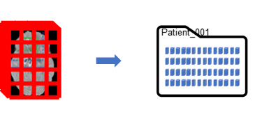
The same analysis was also required for each set of patient data. Each file was required to take a turn being left-out and becoming the test data for cross referencing. There were 36 patient datasets. Each of the 8 training runs is now multiplied 36 times for each left-out file, hence there were a total of 288 training and test runs or experimental trials.

Figure 2. Depiction of Left-One-Out for Channels and Files. Left-Out file used for testing

Figure 3. Final Research Results: Chart on left shows groupings of 36 trials per channel. The chart on the right shows the aggregate results, where a higher value is a better outcome.
Final Exhaustive Experiment Setup and Costs
To accomplish this exhaustive training, the analysis was split over 6 compute instances running in parallel on AWS. On the AWS platform, an instance is a single computer configuration. The Freiburg team first experimented with the more expensive P3 instance types for many training runs before learning that the g4dn’s could be a less costly alternative. The team chose to use the g4dn types. The g4dn's are equipped with single Nvidia Tesla T4 GPU. Each trial took approximately 4 hours, and to complete 288 trials took 8 days. At 0.56 cents per hour for each instance node it cost 1400 dollars. That's probably not too unreasonable, but it took a lot of time and experimenting with failures to build the workflow, determine the best configurations, data storage options, and identify the best Deep Learning parameters. 1000 dollars for each training experiment, not to mention lost time waiting several days for completion will soon become a budget buster.

Figure 4. Depiction of University of Freiburg’s AWS configuration for final experimental run
It takes many iterations of tuning to reach the final training. Understanding the different options on the cloud and how to implement a scalable system and workflow is required to minimize the cost of exhaustive training. A large training effort requires minimizing the time on expensive equipment and minimizing engineering time waiting for completion. There is experimentation with data storage options and minimizing the read times of large datasets, network models, data preprocessing and augmentation, how large of a minibatch the computer configuration can handle, image and image patch sizes, and learning hyperparameters. The Freiburg’s team experiment between the more expensive P3 and the g4dn was such an example.
Workflow
Using Deep network Designer to construct a prototype model
Another experimental phase was choosing network models. The team had become aware of a more recent model, called DeepMedic [2], with some success on brain tissues. They did some initial experimental comparisons with the UNet model and found the DeepMedic required less resources which would hopefully lead to shorter training runs. The team chose to use the two input version of the DeepMedic model, where both inputs are extracted from the same receptive field, but one is processed as a sub-sampled, lower-resolution. Therefore both low-level and high-level details can contribute to the prediction in a more compact model. The subsampled path is up-sampled before the paths are re-combined. The final output is similar to an encoding-only semantic segmentation model. To provide an overlay of the output classes onto the original data, the output has to be scaled to the original data size. See the figure below for a depiction.

Figure 5. Depiction of two input DeepMedic network model
We found we could implement the architecture with a single input and diverging it into two paths with the use of custom cropping layers.

Figure 6. Screen capture of Deep Network Designer (click to enhance)
Since the model was large and there were many duplicate portions, it could be exported at an earlier stage of the build process and then the script could be edited directly, making copying, pasting and name replacement efforts easier. The script could be run when the duplicate parts are completed to generate a model in the workspace for import back to the designer for completion.
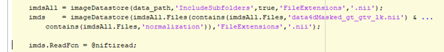
Developing Datastore and Transform Functions for Managing Training and Testing data
Managing and manipulating data sets for deep learning can be very challenging and time consuming. MATLAB uses datastore objects to facilitate Deep Learning. The objects and related constructs support pre- and post-processing, augmentations, background processing and distribution to parallel nodes and GPUs. See Getting Started with Datastores. A folder hierarchy of each patient and their imaging files from each scan event was created. Each MRI scan event contains 7 modalities of different contrasts plus ground truth data. Each scan contains a varying number of slices and varying resolutions. As described earlier, the team was able to implement their own registration and normalization recipe but is out of scope for this blog. imageDatastore was used to access the data. Since the folders were overloaded with multiple data representations and only the normalized files were desired, the datastore list was filtered for files containing the 'normalization' string and the datastore was reconstructed from the resulting list.
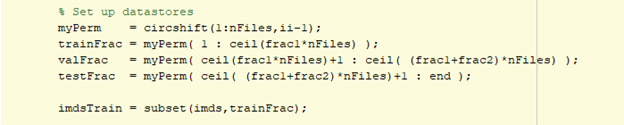
The larger datastore was further subdivided into training, validation, testing datasets using the datastore subset method.
The desired image size for training was on the order of 165x165x9 voxels x 7 channels, which was much smaller than the data in each file. The resolution needed to be retained, otherwise too much information would be lost. For semantic segmentation problems, it is typical to extract random patches from input files that match the training input size. It is also sometimes desired to balance the background voxel counts versus the foreground voxels which has the added benefit of reducing the training time. There is a built-in randamPatchExtractionDatastore to do something similar, but more control was needed for the location of the extractions, the number of reads per file and augmentations. Fortunately, the datastore transform function allows this.
Using BlockedImageDatastore
The research team learned that reading whole files even though only a small portion was required for each read was hampering performance. A work-around was created by creating new datasets from the randomly selected patches. In R2021a, blockedImage and blockedImageDatastore objects were added that improve the performance of these operations. When instantiated, blockedImage will generate a folder of fragment files based on the specified block size. Then only the fragments required for a specified region are read. It will also generate masks and pixel label statistics for each block fragment so regions matching statistical elements can be selected which helps to facilitate balancing of the data for training.
Generating Visualizations
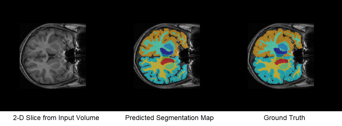
When performing deep learning, visualizing your data can be challenging. MATLAB provides interactive tools to support visualization of volumes and overlaid graphics. Below is an example of using montage to show corresponding slices from each modality, as well as, the ground truth. labeloverlay is used to overlay categorical data on corresponding images. Ground truth and predicted segmentation labels are generally represented as categorical types.

Figure 7. Montage of mid-slice of all 7 Channels/Modalities and ground truth. (Click to enhance image)
Volume Viewer app provides capabilities for selecting and viewing volume slices, with multiple modes for viewing overlaid labels.

Figure 8. VolumeViewer App in Slice Planes mode and Labels mode of T1 channel and ground truth
Using Experiment Manager for Tuning Models
Prior to 2021a, the research team facilitated experiments using nested loops, which can be a tedious way to iteratively train models. After 21a, experimentManager app supplanted scripts the team originally implemented to support Bayesian Optimization and LOO workflows around network training. The purpose of the app is to run experiments with multiple variables, where a range is specified for each variable. In "Sweep" mode, required for LOO analysis, it will run a training trial for each permutation of variables. In "Bayesian" mode it will run a training trial for variable combinations according to the Bayesian optimization algorithm. Below are screen captures from an example based on a 3D Brain Tumor Segmentation example which has similar data to original research. Bayesian and LOO were applied similarly.
 Figure 9. Bayesian Optimization and Sweep Modes Setup panels (click to enhance image) |
 |

Figure 10. Leave-One-Out Training

Figure 11. Bayesian Training. Trial 16 learn rates achieved the best outcome.
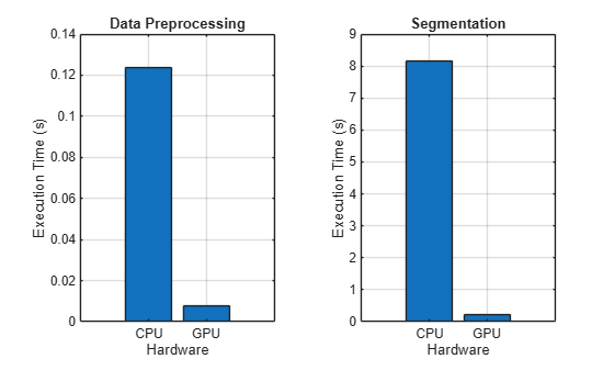
Scaling Up from CPU to GPUs and Cloud Systems
One of the challenges was having a scalable training environment. The research team had limited access to a more powerful single-GPU device and with Parallel Computing Toolbox they could have access to 1,2,4 or 8-GPU devices on AWS. Hence, for general script debugging and limited training the customer would use their personal computer; for more time-intensive workflow troubleshooting and refinement they would schedule time with their in-house single-GPU computer and for heavy-duty training and Bayesian optimization they would target an AWS based multi-GPU instance.
The team decided to use the RDP option. This involved setting up an Amazon Web Service (AWS) account, defining EC2 computing platform instances (charges are per hour) and transferring data to an Elastic Block Storage (EBS). The initial instance is created using a MATLAB Reference Architecture which can then it can be modified for user or application requirements. EBS can be mounted to it or S3 can be accessed as network storage.

See Scale Up Deep Learning in Parallel and in the Cloud for an in-depth discussion in documentation.
A nice feature is that the computer instance configuration (and cost) is easily changed at startup. If training is limited or is still in troubleshooting or refinement mode a lesser instance with a single GPU mode can be selected or when full training is desired the maximum GPUs can be selected and it will finish much more quickly. Learning rates are dependent on minibatch sizes: If it is desired to use the full resource of the GPUs by increasing the minibatch size, then a different learning rate should be considered.
Conclusion
With the new age of AI solutions, there is a lot of research on how to apply it but experimentation is required to identify the best parameters. There was a lot of experimentation to get to the final outcome, i.e. understanding of which modalities were important (See Fig 2). The Freiburg team was able to achieve this by scaling to the cloud, leveraging GPUs and using a variety of apps.
References
[1] Bielak, L., Wiedenmann, N., Berlin, A. et al. Convolutional neural networks for head and neck tumor segmentation on 7-channel multiparametric MRI: a leave-one-out analysis. Radiat Oncol 15, 181 (2020). https://doi.org/10.1186/s13014-020-01618-z [2] Kamnitsas K, Ledig C, Newcombe VFJ, Simpson JP, Kane AD, Menon DK, Rueckert D, Glocker B. Efficient multi-scale 3D CNN with fully connected CRF for accurate brain lesion segmentation. Med Image Anal. 2017;36:61–78 https://doi.org/10.1016/j.media.2016.10.004 Have a question for Arnie? Leave a comment below- Category:
- Deep Learning


Comments
To leave a comment, please click here to sign in to your MathWorks Account or create a new one.