
MathWorks Wins Geoscience AI GPU Hackathon
Background
SEAM (SEG Advanced Modeling Corp.) is a petroleum geoscience industry body that fosters collaborations among industry, government, and academia to address major Geological challenges. Their latest event was a hackathon (SEAM AI Applied Geoscience GPU Hackathon) that sought to explore the use of AI to improve both qualitative and quantitative interpretation of geophysical images of Earth's interior, and speed up the applications using NVIDIA GPUs. A total of 7 teams participated from all over the world, including commercial companies (Chevron, Total, Petrobras) and a mix of industry and university students. Each team was assigned a mentor who is an expert geoscientist working for a top oil and gas company.The Challenge
Geologic interpretation of survey data—especially raw seismic images of Earth's interior is an important step for the oil and gas industry. Seismic images delineate volumes of rock inside the Earth with different physical and geologic characteristics summarized by the term “facies”. An important step in interpretation of the images—which guide exploration, drilling, production, and abandonment of underground reservoirs—is identification and classification of all distinct geologic facies in a seismic image, often called seismic facies identification or classification. This process is still done largely geologists assisted by specialists in geophysical data collection, processing, imaging, and display. Successful interpreters are experts in identifying features such as channels, mass transport complexes, and collapse features. The problem statement of the hackathon was to train an algorithm to recognize distinct geologic facies in seismic images automatically, producing an interpretation that could pass for that of an expert geologist, or be used as a starting point to speed up human interpretation.The Data
We were given the following data set drawn from the Parihaka region off the coast of New Zealand. This data is open to the public and has been labeled by a Chevron geoscientist. The figure below shows a rendering of two vertical slices and one horizontal slice through the 3D seismic image used in this challenge. Standard cartesian coordinate system is used to plot the image, with X and Y measuring the horizontal positions near the earth’s surface and the Z measuring depth below the earth.
Figure 1: 3D views XZ, YZ and XY slices through Parihaka seismic data image (TOP) and corresponding labels (BOTTOM)
The training dataset is a 3D image represented as a matrix of size 1006 x 782 x 490 real numbers stored in the order or (Z,X,Y). Labels corresponding to the training data are similarly arranged and consists of integers with values ranging between 1 to 6. Figure 2 below shows the intensity plot of the echoes and the corresponding labels for each pixel in one 2D cross-sectional view of an XZ slice.
Figure 2: 2D cross-sectional view of XZ slice (LEFT), and pixel-by-pixel classification of image in 6 facies (RIGHT)
Our Approach
Most of the current techniques for automated seismic facies labeling were using convolution neural networks for semantic segmentation [1][2][3]. However, many of these methods had an issue of overfitting, and mentioned that the trained algorithm was only applicable to the survey region in proximity to the model training dataset. If the algorithm was used on a dataset from a different geographic location, the model would likely need retraining. We wanted to leverage the work already done in this domain and come up with a technique which is less susceptible to overfitting and could be applied to a much wider geographical area without the need of retraining. That is when we thought of taking a signal-based approach: since the 3D image volume is constructed from 1D echo signals, perhaps there is some potential of leveraging the unique signatures of these echoes across different facies. Figure 3 shows a small section of the 2D image with signals superimposed on the facies. Upon close inspection we can see that each signal, also referred to as a "trace", has a distinct signature when it encounters different facies. For instance, at the transition from "dark blue" to "green" facies in the middle of image, the signal has a burst of high echo-amplitudes rapidly oscillating, whereas the interface below that between "light blue" and "dark blue" region has slower oscillations with a lower amplitude. Expert geologists often look for these features in the vertical sequence of pixel values to identify the key interfaces between different facies.
Figure 3: Plots of image values (red) as a function of depth, superimposed on the facies interpretation in a small section. Note that that a burst of high echo-amplitudes rapidly alternating between positive and negative values is characteristic of the transition between “blue” and “green” facies across the middle part of the image.
Next, we used a Recurrent Neural Network (RNN) architecture to train a sequence-by-sequence classification network using the input traces, but in our preliminary attempts the network was failing to converge. This was primarily due to the signal length being is quite long and the distinct signal features changing very rapidly with time. If we could separate the unique facies signatures into separate channels, we might have a better chance of training the network. We decided to utilize a wavelet multiresolution analysis technique: multi-resolution analysis (MRA) uses discrete wavelet transform to break the signal into components which decomposes the variability of the data into physically meaningful and interpretable parts. In our case we used MRA directly from Signal Multiresolution App in MATLAB, and after experimenting through various discrete wavelets, we got the best decomposition results with ‘fk14’ wavelet and divided the signal into 5 levels.
Figure 4: Multiresolution decomposition of the original signal into four levels + Approximation using fk14 wavelet. This is done using Signal Multiresolution App in MATLAB
We also generated MATLAB code directly from this app by selecting the export option, to apply the same wavelet decomposition with MRA on all signals.% load the training data and labels load data_train.mat; load labels_train.mat; % Convert the data to double and labels to categorical datatype data = double(data); labels = categorical(labels); % Apply the maximal overlap discrete wavelet transform on all traces dataMRA = zeros([size(data),5]); parfor ii = 1 : 782 for jj = 1:590 dataMRA(:,ii,jj,:) = modwt(data(:,ii,jj), 'fk14',4)'; end endNow we have 5 channels for each trace. To capture the correlation of nearby traces we grouped 3x3 traces in the XY plane together and used that to train the same labels of the middle trace. This was done assuming the signals resolution in the XY plane is low enough that the seismic features do not change across 3x3 sample grid. Figure 5 shows how the dataset was grouped into 3X3 grid for 5 channels for each trace.

Figure 5: Arranging the data into training set
dataTrain = {};
labelsTrain = {};
for ii = 2: 782-1
    for jj = 2:590-1
      tempData = permute((dataMRA(:,ii-1:ii+1, jj-1:jj+1, :)), [1 4 2 3]);
      dataTrain(ii+jj-3,1) = {reshape(tempData, [1006 45])'} ;
      labelsTrain(ii+jj-3,1) = {labels(:,ii,jj)'};
    end
end
At this stage we also divided our dataset into training and validation sets to be used during training. To make our network robust, we randomly chose 1000 traces out of 782x590 traces for training and used the remaining for network validation.
idx = randperm(size(dataTrain,1));

% Train data and labels
trainData = dataTrain(idx(1:1000));
valData = dataTrain(idx(1001:end));

% Test data and labels
trainLabel= labelsTrain(idx(1:1000));
valLabel = labelsTrain(idx(1001:end));
Next, we were ready to architect our deep learning network for training. The dataset was arranged to feed into an RNN sequence-by-sequence in the Z direction. Initially we started with Long Short-Term Memory (LSTM) layers but after a few iterations realized that a Gated Recurrent Unit (GRU) layer was giving us a better performance. The deep learning layers were constructed using Deep Network Designer app in MATLAB and analyzed using the network analysis tool. Figure 6 shows the full architecture of the network on Deep Network Analyzer App and its analysis. If you look at the network, we have the first layer being Sequence Input layer with an input size of 45 (3x3x5 channels), and the final classification layer is of size 6x1 corresponding to the scores it will predict for each label class.

Figure 6: Deep Network Designer App to architect the RNN layers (top) and the network analysis (bottom)
We can directly generate the MATLAB code for the layer architecture by exporting code from the app.inputSize = [45];
numHiddenUnits1 = 20;
numHiddenUnits2 = 30;
numClasses = 6;
GRUlayers = [ ...
sequenceInputLayer(inputSize,'Name','InputLayer',...
'Normalization','zerocenter')
gruLayer(numHiddenUnits1,'Name','GRU1','OutputMode','sequence')
dropoutLayer(0.35,'Name','Dropout1')
gruLayer(numHiddenUnits2,'Name','GRU2')
dropoutLayer(0.2,'Name','Dropout2')
fullyConnectedLayer(numClasses,'Name','FullyConnected')
softmaxLayer('Name','smax');
classificationLayer('Name','ClassificationLayer')];
After this step, we defined the training options, for deep network training. The training was performed on a single NVIDIA Ampere A100 GPU using the MATLAB AWS Reference architecture cloud image. Figure 7 shows the deep learning training progress.
maxEpochs = 300;
miniBatchSize = 15;

options = trainingOptions('adam', ...
    'ExecutionEnvironment','auto', ...
    'L2Regularization',1e-3,...
    'InitialLearnRate',1e-3, ...
    'MaxEpochs',maxEpochs, ...
    'MiniBatchSize',miniBatchSize, ...
    'Shuffle','every-epoch',...
    'Verbose',0,...
    'Plots','training-progress', ...
    'ValidationData', {valData, valLabel});

[netGRU,infoGRU] = trainNetwork(dataTrain,labelsTrain,GRUlayers,options);

Figure 7: Training progress for deep learning network
Results
The competition ran for a duration of 2 weeks, and the results were declared on April 22nd 2021. The competition had several highs and lows. We literally had 3 sleepless nights on the weekend before the submission. We had to iterate over different approaches before we came up with our final solution. We initially started out with training LSTMs on raw signal and gradually kept adding additional techniques, before coming up with the final solution. There were 3 metrics to judge the quality of submission:- Facies-weighed F1 score with different weighting among the facies: Highest weights for facies 5 and 6 since these were geologically most important.
- Facies-weighted percentage of pixels correct: Highest weights for facies 5 and 6 since these were geologically most important.
- Interface-weighted F1-score: F1-score is calculated for each pixel, with pixels within 10 samples of an interface were given 20 times the weight of all other samples.

Figure 8: Leaderboard for the results with MathWorks having the top score. Note the F1-Weighted score discrepancy between MathWorks and other teams!

Figure 9: Weighted F1 score calculated for test dataset
What's Next
- We now have a novel fully functioning solution to seismic facies classification problem (we'll be happy to send you code if you reach out to deep-learning@mathworks.com). We strongly believe this approach will help overcoming the limitations with convolution neural networks.
- We will combine the CNNapproach [1][2] with the RNN deep learning network approach with a goal to get the best prediction with both images and signals approach. Figure 10 shows the future work architecture, where we would train two different 2D UNets across the XZ and YZ plane and combine it with the RNN network predictions. For each trace we would have classifications from 3 networks, and a pooling algorithm will analyze the scores and pick out the final prediction class.

Figure 10: Future work to combine UNet with RNN for facies classification
References
[1] Liang-Chieh Chen, George Papandreou, Iasonas Kokkinos, Kevin Murphy, and Alan L Yuille. Deeplab: Semantic image segmentation with deep convolutional nets, atrous convolution, and fully connected crfs. IEEE transactions on pattern analysis and machine intelligence, 40(4):834–848, 2018b. [2] Zengyan Wang, Fangyu Li, Thiab R. Taha and Hamid R. Arabnia. Improved Automating Seismic Facies Analysis Using Deep Dilated Attention Autoencoders. Conference: 2019 IEEE/CVF Conference on Computer Vision and Pattern Recognition Workshops (CVPRW) [3] Geng, Z., Wang, Y. Automated design of a convolutional neural network with multi-scale filters for cost-efficient seismic data classification. Nat Commun 11, 3311 (2020). https://doi.org/10.1038/s41467-020-17123-6- Category:
- Deep Learning


Comments
To leave a comment, please click here to sign in to your MathWorks Account or create a new one.