
Time Series Analysis of Trends in Global Carbon Emissions from Fossil Fuels
The following post is from Hang Qian, Software Developer on the Econometrics Toolbox Team.
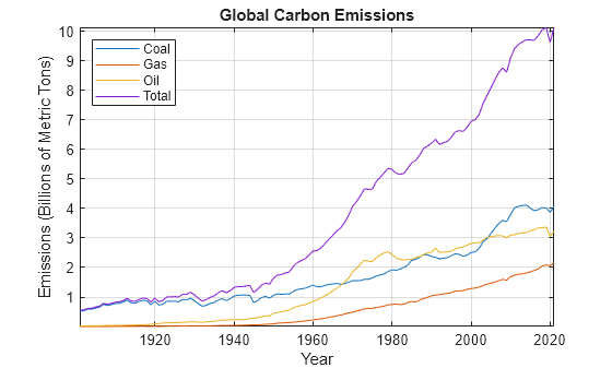
Global carbon emissions have increased dramatically since 1901. However, the annual growth rates were time-varying in the past century and slowed down in recent years, possibly due to international efforts on climate change under the Kyoto Protocol and Paris Agreement, and exogenous shocks by the pandemic.
This demo analyzes time-varying local trends of carbon emissions from fossil fuels and builds a multivariate dynamic factor model for carbon emissions from coal, gas, and oil.
Retrieve Data from Haver Analytics®
The Datafeed Toolbox™ enables you to connect to Haver Analytics databases to retrieve their economic data for analysis in MATLAB®.
Connect to the Haver Analytics Environmental, Social, and Governance Indicators (ESG) database by specifying its database name file located on your local machine, for example, C:\DLX\DATA\ESG.dat.
h = haver(“C:\DLX\DATA\ESG.dat”);
h.DataReturnFormat = “timetable”;
The ESG database contains yearly measurements of carbon emissions from burning fossil fuels from 1901, among other series.
- C001BB — Total yearly carbon emissions from burning fossil fuels (billions of metric tons of CO2)
- C001BBTP — Carbon-emission contribution from coal
- C001BBTG — Carbon-emission contribution from gas
- C001BBTO — Carbon-emission contribution from oil
CO2Emissions = fetch(h,[“C001BB” “C001BBTP” “C001BBTO” “C001BBTG”]);
CO2Emissions is a 4-column cell array containing timetable objects with the carbon-emission measurements for each retrieved series.
Visualize the Time Series
Specify variables for each time series.
dates = CO2Emissions{1}.Time;
fossil = CO2Emissions{1}.GlobalCarbonEmissionsFromFossilFuelCombustion_Industry_Bil_Metr;
coal = CO2Emissions{2}.GlobalCarbonEmissionsFromCoal_Bil_MetricTons_;
oil = CO2Emissions{3}.GlobalCarbonEmissionsFromOil_Bil_MetricTons_;
gas = CO2Emissions{4}.GlobalCarbonEmissionsFromGas_Bil_MetricTons_;
Visually inspect the variables to determine their dynamic properties.
figure
tl = tiledlayout(4,1);
nexttile
plot(dates,coal)
title(“Coal”)
nexttile
plot(dates,oil)
title(“Gas”)
nexttile
plot(dates,gas)
title(“Oil”)
nexttile
plot(dates,fossil)
title(“Fossil”)
xlabel(tl,“Year”);
ylabel(tl,“Carbon Emissions (bil. metric tons)”);
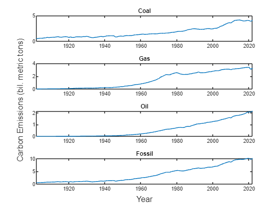
The time series plots indicate that carbon emissions have an upward trend, but a deterministic linear trend is inadequate for time series modeling.
Estimate Local-Trend State-Space Model

The local function paramMap is a parameter mapping function that defines the local trend model of a single variable in state-space form. Create a state-space model by passing the parameter mapping paramMap to ssm and estimate the unknown parameters by maximum likelihood using estimate.
Mdl = ssm(@paramMap);
y = fossil;
params0 = [0.1; 0.1; 0.5; 0.01];
EstMdl = estimate(Mdl,y,params0,Univariate=true,lb=zeros(4,1));
Based on the fitted model, the Kalman filter and smoother provide the state estimation. The first state variable corresponds to the local trend, and the second variable is the lagged variable.
States = smooth(EstMdl,y);
localTrend = States(:,1);
Forecast Local-Trend State-Space Model
The estimated local trend facilitates the out-of-sample forecast. Without new observations, assume that the current state of the growth momentum passes on to the forecasting periods. The Kalman filter provides the forecasted carbon emission levels.
Forecast the local trend model into a horizon of length n. Compute approximate 95% forecast intervals. Plot the forecasts.
n = 10;
[yf,yfMSE] = forecast(EstMdl,n,y);
yfLB = yf – 2*sqrt(yfMSE);
yfUB = yf + 2*sqrt(yfMSE);
xf = datetime((year(dates(end))+1:year(dates(end))+n)’,1 ,1);
figure
plot(dates,y,“-b”, …
dates,localTrend,“–m”, …
xf,yf,“.b”, …
xf,yfLB,“–r”, …
xf,yfUB,“–r”);
xlabel(“Year”)
ylabel(“Carbon Emissions (bil. metric tons)”)
title(“In-Sample Fit and Out-of-Sample Forecast”)

Dummy Variables for Intervention Effects
As countries are working towards carbon neutrality, it is of interest to consider the effects of the Kyoto Protocol and the Paris Agreement on carbon emissions. Also, exogenous shocks by the pandemic slowed down the world economy, which resulted in the reduction of greenhouse gas emissions. Create dummy variables that indicate interventions on climate.
Kyoto = year(dates) > 1997;
Paris = year(dates) > 2015;
Covid = year(dates) >= 2020;
Dummy = [Kyoto Paris Covid];
nvar = size(Dummy,2);
The local function paramMapDummy is a parameter mapping that includes the exogenous predictors in the observation equation of the local-trend state-space model. Create a state-space model for the local-trend model with intervention dummy variables, and then fit the model to the total carbon emissions variable fossil.
MdlDummy = ssm(@(params)paramMapDummy(params,fossil,Dummy));
params0Dummy = [params0; zeros(nvar,1)];
[~,estParams] = estimate(MdlDummy,fossil,params0Dummy, …
Univariate=true,lb=[zeros(4,1); -Inf(nvar,1)]);
The last three parameters correspond to the intervention effects. Empirical results confirm that carbon emissions have been reduced under the Kyoto Protocol and Paris Agreement. The pandemic also has a significant negative effect on greenhouse gas emissions.
disp(estParams(5:7)’)
Common Local Trend for Three Series
Assume that a common stochastic trend drives global carbon emissions from coal, gas, and oil. This is a dynamic factor model, in which the common local trend serves as an unobserved factor underlying three observed time series. To prepare for the multivariate extension of the local trend model, reparametrize the local trend as

Y = [coal oil gas];
MdlFactor = ssm(@(params)paramMapFactor(params,Y));
params0Factor = [0.1*ones(3,1); 0.1*ones(3,1); 0.5; 0.01];
estimate(MdlFactor,Y,params0Factor,Univariate=true, …
lb=zeros(size(params0Factor)));
Conclusion
A feature of the state-space model is to incorporate the unobserved components like local levels and trends in the state variables. As a nonstationary model, the random-walk local trend captures the time-varying trends that provide a good fit for the global carbon emission data.
Local Functions
function [A,B,C,D,mean0,Cov0] = paramMap(params)
sigmaU = params(1);
sigmaE = params(2);
intercept = params(3);
slope = params(4);
A = [2 -1;1 0];
B = [sigmaU;0];
C = [1 0];
D = sigmaE;
mean0 = [intercept;intercept-slope];
Cov0 = zeros(2);
end
function [A,B,C,D,mean0,Cov0,stateType,yDeflate] = paramMapDummy(params,y,Dummy)
sigmaU = params(1);
sigmaE = params(2);
intercept = params(3);
slope = params(4);
dummyCoeff = params(5:end);
A = [2 -1;1 0];
B = [sigmaU;0];
C = [1 0];
D = sigmaE;
mean0 = [intercept;intercept-slope];
Cov0 = zeros(2);
stateType = [2;2];
yDeflate = y – Dummy*dummyCoeff;
end
function [A,B,C,D,mean0,Cov0,stateType,YDeflate] = paramMapFactor(params,Y)
sigmaU = params(1:3);
sigmaE = params(4:6);
intercept = params(7);
slope = params(8);
A = [2 -1;1 0];
B = [1;0];
C = [sigmaU, zeros(3,1)];
D = diag(sigmaE);
mean0 = [0;0];
Cov0 = zeros(2);
stateType = [2;2];
linear = [intercept;0;0] + [slope;0;0] .* (1:size(Y,1));
YDeflate = Y – linear’;
end
- Category:
- Climate Finance,
- Econometrics,
- New Features


Comments
To leave a comment, please click here to sign in to your MathWorks Account or create a new one.