
Multi-Armed Bandit Problem and Exploration vs. Exploitation Trade-off
Casino slot machines have a playful nickname - "one-armed bandit" - because of the single lever it has and our tendency to lose money when we play them. They also inspire the creativity of researchers. Today's guest blogger, Toshi Takeuchi, will introduce an interesting thought experiment known as multi-armed bandits.
Ordinary slot machines have only one lever. What if you had multiple levers to pull, each with different payout. This is a multi-armed bandit. You don't know which lever has the highest payout - you just have to try different levers to see which one works best, but for how long? If you keep pulling the low payout lever, you forego more rewards, but you won't know which lever is good until you try a sufficient number of times.
This interesting thought experiment, originally developed during World War II, was so intractable that allied scientists wanted to drop this problem over Germany so that German scientists could also waste their time on it. Since then, a number of strategies have been developed to solve this problem, but apparently many people are still working on it given the number of papers on this topic in NIPS 2015.
This is because bandit algorithms are related to the field of machine learning called reinforcement learning. Rather than learning from explicit training data, or discovering patterns in static data, reinforcement learning discovers the best option from trial and error with live examples. The multi-armed bandits in particular focus on the question of exploration vs. exploitation trade-off - how many resources should be spent in trial and error vs. maximizing the benefit.
Contents
- Example - Choosing the Optimal Color for Buy Now Button
- Epsilon-Greedy Strategy
- Testing Button Colors with a Three-Armed Bandit
- The First Trial
- Repeat Trials
- Estimated vs. Actual Expected Rewards
- Regret
- Creating Live Demo
- Epsilon-Decreasing Strategy
- Test the New Strategy
- Updating the Live Demo
- Real World Uses
- Summary - Is life a bandit problem?
Example - Choosing the Optimal Color for Buy Now Button
Let's take a look at a couple of the basic popular strategies here using an example from a blog post 20 lines of code that will beat A/B testing every time. It talks about how you can use bandit algorithms instead of plain vanilla A/B testing in website optimization and provides a concise pseudo code.
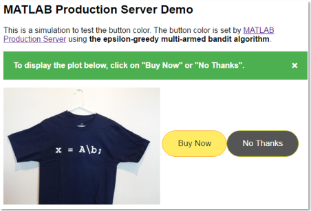
We will use an example similar to the one used in the blog post: should a "Buy Now" button be colored blue, orange, or yellow, to maximize the clicks? You can see a live demo of this problem in action powered by MATLAB Production Server running on AWS.
Epsilon-Greedy Strategy
This strategy lets you choose an arm at random with uniform probability for a fraction $\epsilon$ of the trials (exploration), and the best arm is selected $(1 - \epsilon)$ of the trials (exploitation). This is implemented in the eGreedy class as the choose method. The usual value for $\epsilon$ is 0.1 or 10% of the trials.
What is the "best" arm? At each trial, the arm we choose to pull may or may not give a reward. The best arm has the highest expectation of reward based on the rewards received up to that point. We keep track of the expected rewards for respective arms as scores.
dbtype 'eGreedy.m' 31:38
31            function choice = choose(self)          % choose an arm
32                if rand <= self.epsilon             % (epsilon) times
33                    choice = randi(self.n_arms);    % explore all arms
34                else                                % (1 - epsilon) times
35                    [~, choice] = ...               % exploit the best arm
36                        max(self.scores(end,:));
37                end
38            end
Testing Button Colors with a Three-Armed Bandit
In our example, we can think of those buttons as choices of levers we can pull, and we get a reward of click or no click with an unknown probability with each color. This is known as a binary reward. The bandit class creates an object with three arms with unknown probabilities, which in this case represent respective "Buy Now" buttons. Let's call that object buttons. The object provides the test method that returns a reward of 1 or 0 for a chosen button we show, which represents a click (1) or no click (0).
We will estimate the unknown click probabilities of those buttons through our trials using the eGreedy class, which we will initialize as the myGreedy object with $\epsilon$ set to 0.1 by default. Initial expected rewards are also set uniformly to 1 for all arms, which means we expect buttons to get clicked 100% of times.
cols = {'Blue','Orange','Yellow'};          % button colors as arms
buttons = bandit();                         % initialize bandit with 3 arms
myGreedy = eGreedy(buttons.N);              % epsilon-greedy with epsilon = 0.1
s = array2table(myGreedy.scores);           % initial expected reward
s.Properties.VariableNames = cols           % name columns by color
s =
    Blue    Orange    Yellow
    ____    ______    ______
    1       1         1
The First Trial
In trials, we will choose a button based on the epsilon-greedy strategy using the choose method in the myGreedy object. Because the initial expected rewards are uniformly set to 1, one of the three colors will be selected randomly when a web visitor comes to a page.
rng(1);                                     % for reproducibility
color = myGreedy.choose()                   % choose a button color
color =
     1
We will then display the blue button to the visitor on the page and this is implemented using the test method, which is equivalent to pulling the lever on a slot machine. The reward (click) is given with the hidden probability of the chosen button.
click = buttons.test(color) % display the button
click =
  logical
   0
Based on the actual result, we will update our expected reward for the chosen button. Since we didn't get the reward with the blue button, the expected reward for that button is now reduced: $Blue = 1/2 = 0.5$
myGreedy.update(color, click);              % update expected reward
s = array2table(myGreedy.scores);           % new expected reward
s.Properties.VariableNames = cols;          % name columns
s.Properties.RowNames={'Initial','Trial_1'} % name rows
s =
               Blue    Orange    Yellow
               ____    ______    ______
    Initial      1     1         1
    Trial_1    0.5     1         1
Repeat Trials
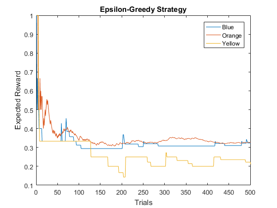
Let's continue for more trials and plot the changes in expected rewards. Initially the values fluctuate a lot, but eventually they settle into certain ranges. It looks like orange has the highest expected reward and blue has a slightly lower one.
n_trials = 500;                             % number of trials
for i = 1:n_trials - 1                      % subtract completed trial
    color = myGreedy.choose();              % choose a color
    click = buttons.test(color);            % test the button
    myGreedy.update(color, click);          % update expected reward
end
name = 'Epsilon-Greedy Strategy';           % title
myGreedy.plot(name, cols)                   % plot expected rewards
Estimated vs. Actual Expected Rewards
We will never know the actual probabilities in real world situations, but this is just a simulation, so we know the actual parameters we used to generate random rewards. Let's see how close we came to estimating them using the epsilon-greedy strategy. The estimates are off, but it still managed to identify the best button correctly.
array2table([myGreedy.scores(end,:); buttons.probs], ...
    'VariableNames',cols, ...
    'RowNames',{'Estimated','Actual'})
ans =
                  Blue      Orange     Yellow
                 _______    _______    _______
    Estimated    0.32353    0.32667    0.21053
    Actual          0.28       0.32       0.26
Regret
Let's consider alternative scenarios. Had we done this test under a standard A/B testing protocol, we would have shown three buttons with equal proportions first to pursue pure exploration and then switch to pure exploitation by only showing the best button. This is also known as the epsilon-first strategy. Let's assume we did the A/B testing with the first 300 trials and only showed the orange button thereafter.
Had we known the best button to use ahead of time, we would have shown the orange button all the time as the optimal strategy.
strategies =  {'Epsilon-First','Epsilon-Greedy','Optimal'};
trials = array2table([100 300 100; ...      % number of trials
    myGreedy.trials; [0 n_trials 0]]);
trials.Properties.VariableNames = cols;     % name cols
trials.Properties.RowNames = strategies     % name rows
trials =
                      Blue    Orange    Yellow
                      ____    ______    ______
    Epsilon-First     100     300       100
    Epsilon-Greedy     33     449        18
    Optimal             0     500         0
We can calculate the expected clicks (rewards) from each strategy and see how many fewer clicks we got using the epsilon-greedy vs. the epsilon-first (A/B testing). These differences are known as "regrets". You can see that the epsilon-greedy came pretty close to the optimal.
clicks = sum(bsxfun(@times, ...             % get expected number
    table2array(trials), buttons.probs), 2);% of clicks
Regret = clicks - clicks(end);              % subtract optimal clicks
Regret =  table(Regret, 'RowNames', strategies)
Regret =
                      Regret
                      ______
    Epsilon-First      -10
    Epsilon-Greedy    -2.4
    Optimal              0
Creating Live Demo
My colleague Arvind Hosagrahara in consulting services helped me to create the live demo linked earlier. Please read Arvind's excellent blog post Build a product, build a service for more details about how to create a web app with MATLAB. Here is the quick summary of what I did.
- Create two wrapper functions pickColor and scoreButton to call my eGreedy class
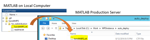
- Compile the wrapper functions with eGreedy and other dependencies into a CTF file with MATLAB Compiler SDK
- Deploy the CTF file to Mthe ATLAB Production Server Arvind is running on AWS by uploading the file
- Create the web front end on jsFiddle (See the source code, particularly the JAVASCRIPT section)
Don't worry if you don't understand JavaScript. In a real world project, you would work with a team of web developers and IT people and they will take care of the web front end and IT back end, and you can just focus on your MATLAB code. The beauty of this approach is that you can use your MATLAB code directly itself, rather than re-doing it in C/++, .NET or Java.
Epsilon-Decreasing Strategy
Now back to the algorithm. One issue with the epsilon-greedy strategy is how to set the value of $\epsilon$, and how we continue exploring suboptimal arms at that rate even after the algorithm identifies the optimal choice. Rather than using a fixed value for $\epsilon$, we can start with a high value that decreases over time. This way, we can favor exploration initially, and then favor exploitation later on. We can easily create a new class eDcrease from eGreedy to accomplish that.
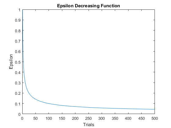
The tricky part is how we should define our function that decreases the $\epsilon$ value. Here is one way of doing it. It starts with pure exploration but we allocate more trials for exploitation as the experiment progresses, with gradually decreasing s of $\epsilon$ . I tried different decreasing functions but it seems like the rate of decrease shouldn't be too quick to get the best result.
f = @(x) 1 ./ (x .^ .5);                    % decreasing function
x = 1:n_trials;                             % number of trials
figure                                      % new figure
plot(x,f(x))                                % plot epsilon value
xlabel('Trials')                            % x-axis label
ylabel('Epsilon')                           % y-axis label
title('Epsilon Decreasing Function')        % title
Test the New Strategy
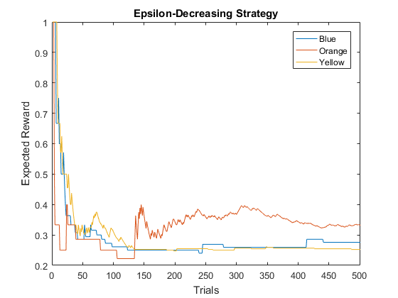
Let's now run this for the same number of trials. It looks like it also identified the orange button as the best option, but it spent more time in exploration initially.
rng(1);                                     % for reproducibility
myDec = eDecrease(buttons.N, f);            % initialize object
for i = 1:n_trials                          % repeat trials
    color = myDec.choose();                 % choose a color
    click = buttons.test(color);            % test the button
    myDec.update(color, click);             % update expected reward
end
name = 'Epsilon-Decreasing Strategy';       % title
myDec.plot(name, cols)                      % plot expected rewards
The estimated expected rewards are also closer to the actual values.
array2table([myDec.scores(end,:);buttons.probs], ...
    'VariableNames',cols, ...
    'RowNames',{'Estimated','Actual'})
ans =
                  Blue      Orange     Yellow
                 _______    _______    _______
    Estimated    0.27586    0.33148    0.25217
    Actual          0.28       0.32       0.26
Unfortunately, the result shows that this strategy is not doing as well as the epsilon-greedy one.
strategies =  {'Epsilon-First','Epsilon-Greedy','Epsilon-Decreasing','Optimal'};
trials = array2table([[100 300 100]; ...    % number of trials
    myGreedy.trials; myDec.trials; [0 n_trials 0]]);
clicks = sum(bsxfun(@times, ...             % get expected number
    table2array(trials), buttons.probs), 2);% of clicks
Regret = clicks - clicks(end);              % subtract optimal clicks
Regret =  table(Regret, 'RowNames', strategies)
Regret =
                          Regret
                          ______
    Epsilon-First           -10
    Epsilon-Greedy         -2.4
    Epsilon-Decreasing    -7.96
    Optimal                   0
Updating the Live Demo
If the epsilon-decreasing strategy had worked, I might have wanted to update my live demo. Had I implemented the epsilon-greedy algorithm in other languages, I would have had to re-code all over again. Luckily, I am using my original MATLAB code, so this is what I would do:
- Change the wrapper functions to call eDecrease rather than eGreedy and re-deploy them to MATLAB Production Server.
- No change to the web front end
- No change to the IT back end
If you are working in a team, this means you can update your code freely without asking your front end or back end people to help you out. Sweet! This is a powerful workflow advantage you gain from using MATLAB Production Server.
Real World Uses
In the examples we used here, we consider the case of choosing the best color for the "Buy Now" button on a web page but you can see this would be useful, for example, to choose which ads a news aggregator website should show on the search page - the Washington Post apparently uses a bandit algorithm for that.
Recommender systems typically face the cold start problem - for example, Netflix has no data for how people would rate newly released movies. It can still recommend such movies through a trial and error process as well.
We also talked about the advantage of MATLAB Production Server in your workflow. One of the pain points Netflix experienced is the problem of dual implementations - you prototype your algorithm in one language such as MATLAB, and you deploy it to production systems in another - such as C/C++, .NET, or Java. This means you have to re-code every time you change your algorithm. You can prototype your algorithm in MATLAB, and that code can be deployed to production system quite easily with MATLAB Production Sever.
Summary - Is life a bandit problem?
MATLAB Community blog host Ned saw an early draft of this post and sent me this video about using algorithms to make life decisions like when to stop looking for an ideal apartment or spouse. It is a different genre of algorithm called optimal stopping, but the video proposes that you can apply it in life. Maybe you can also find a way to apply bandit algorithms in life. Let us know how you would use this algorithm here!
- Category:
- Deployment,
- Statistics


Comments
To leave a comment, please click here to sign in to your MathWorks Account or create a new one.