
Down the Tubes (Parametric Curves Part 2)
The ribbons we created last time are nice, but sometimes we want something a bit more solid. Something like a tube.
To do that, a single vector normal to the curve is not going to be sufficient. We need two vectors which are normal to the curve and also normal to each other. In theory the third partial (aka the binormal) fits the bill, but it tends to behave rather poorly in practice.
Another approach is to use the cross product. Remember that if we compute the cross product of two vectors, we get a third vector which is normal to each of those. This means that if we cross the tangent and the normal vectors that we computed last time, we'll get another vector with exactly the behavior we need. We can do that with this function.
function [xo,yo,zo] = cross_vectors(x1,y1,z1, x2,y2,z2)
  n = numel(x1);
  xo = zeros(1,n);
  yo = zeros(1,n);
  zo = zeros(1,n);
  for i=1:n
    xo(i) = y1(i)*z2(i) - z1(i)*y2(i);
    yo(i) = z1(i)*x2(i) - x1(i)*z2(i);
    zo(i) = x1(i)*y2(i) - y1(i)*x2(i);
  end
Which we can use like this:
t = 0:pi/128:2*pi;
x = 3*cos(t)+cos(10*t).*cos(t);
y = 3*sin(t)+cos(10*t).*sin(t);
z = sin(10*t);
Get the tangent vector.
dxdt = -3*sin(t) - cos(10*t).*sin(t) - 10*sin(10*t).*cos(t);
dydt = 3*cos(t) + cos(10*t).*cos(t) - 10*sin(10*t).*sin(t);
dzdt = 10*cos(10*t);
Get the normal vector.
d2xdt2 = -3*cos(t) + 20*sin(10*t).*sin(t) - 101*cos(10*t).*cos(t);
d2ydt2 = -3*sin(t) - 101*cos(10*t).*sin(t) - 20*sin(10*t).*cos(t);
d2zdt2 = -100*sin(10*t);
[n1x,n1y,n1z] = normalize_vector(d2xdt2,d2ydt2,d2zdt2);
And cross them to get a second normal vector.
[cx,cy,cz] = cross_vectors(dxdt,dydt,dzdt, d2xdt2,d2ydt2,d2zdt2);
[n2x,n2y,n2z] = normalize_vector(cx,cy,cz);
plot_vectors(x,y,z, n1x,n1y,n1z);
hold on
plot_vectors(x,y,z, n2x,n2y,n2z);
set(gca,'DataAspectRatio',[1 1 1])
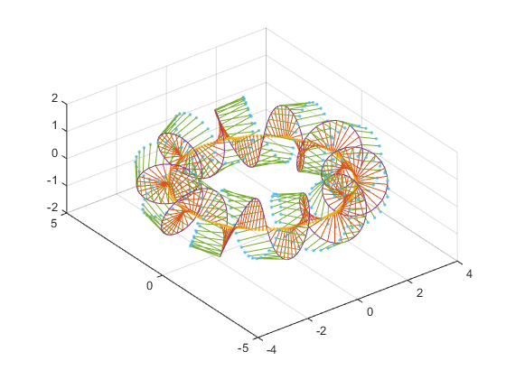
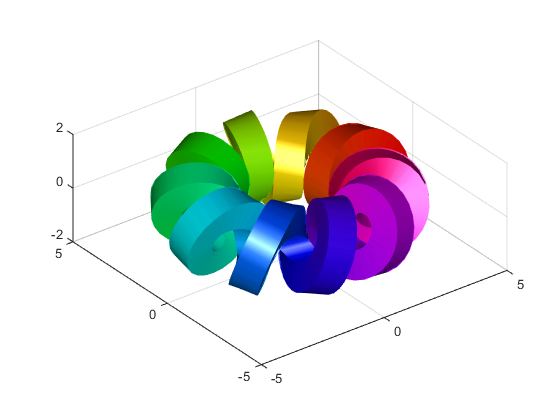
Now we have two sets of normals which we can use to create four ribbons which make a closed tube around the curve. Notice the pattern here. We create 4 ribbons. Each one uses one of our 2 vectors in either the + or - direction, and then creates 2 rows from the + and - versions of the "other" vector.
sides = gobjects(1,4);

sx = [x+(-n1x-n2x)/2; x+( n1x-n2x)/2];
sy = [y+(-n1y-n2y)/2; y+( n1y-n2y)/2];
sz = [z+(-n1z-n2z)/2; z+( n1z-n2z)/2];
sides(1) = surf(sx,sy,sz,[t;t]);
hold on

sx = [x+( n1x-n2x)/2; x+( n1x+n2x)/2];
sy = [y+( n1y-n2y)/2; y+( n1y+n2y)/2];
sz = [z+( n1z-n2z)/2; z+( n1z+n2z)/2];
sides(2) = surf(sx,sy,sz,[t;t]);

sx = [x+( n1x+n2x)/2; x+(-n1x+n2x)/2];
sy = [y+( n1y+n2y)/2; y+(-n1y+n2y)/2];
sz = [z+( n1z+n2z)/2; z+(-n1z+n2z)/2];
sides(3) = surf(sx,sy,sz,[t;t]);

sx = [x+(-n1x+n2x)/2; x+(-n1x-n2x)/2];
sy = [y+(-n1y+n2y)/2; y+(-n1y-n2y)/2];
sz = [z+(-n1z+n2z)/2; z+(-n1z-n2z)/2];
sides(4) = surf(sx,sy,sz,[t;t]);

hold off
set(sides,'EdgeColor','none');
set(sides,'FaceColor','interp');
set(sides,'FaceLighting','gouraud');
set(gca,'DataAspectRatio',[1 1 1])
colormap(hsv(256))
camlight headlight
That looks pretty good, but let's take a closer look. What if we move the camera inside the scene and use a perspective projection? While we're at it, let's save it to an animated GIF.
a = gca;
a.Visible = 'off';
a.Projection = 'perspective';
a.CameraViewAngle = 45;
first = true;
for theta=t
    a.CameraPosition = 3*[cos(theta), sin(theta), 0];
    a.CameraTarget = a.CameraPosition + [-sin(theta), cos(theta), 0];
    im = getframe(gcf);
    [A,map] = rgb2ind(im.cdata,256);
    if first
        first = false;
        imwrite(A,map,'torus_animation.gif','LoopCount',Inf,'DelayTime',1/24);
    else
        imwrite(A,map,'torus_animation.gif','WriteMode','append','DelayTime',1/24);
    end
end
- Category:
- Geometry

