
Patch Work
Patch Work
Back before the internet, programmers collected xeroxed copies of old notes and papers. We traded these with our friends and coworkers, like samizdat. I still have a large filing cabinet full of these.
One of my favorites is:
  Patch Work
  Rob Cook
  Technical Memo #118
  Computer Division
  Lucasfilm Ltd
You can find some of the other old Lucasfilm technical memos in Pixar's library. But as far as I know, this one has never appeared on the internet.
The "Patch Work" memo was a collection of useful tidbits about the different types of patches which were used for representing smooth surfaces. Rob collected these from work that had been done by Loren Carpenter, Ed Catmull, and Tom Duff. If you worked with surface patches, it was really handy to have a single, short memo with all of this useful information collected in one place. That made this one of the more valuable graphics samizdats.
Let's take a quick look at some of what's in this wonderful old memo.
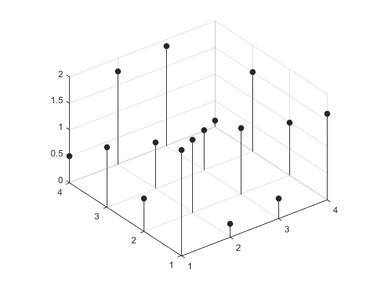
First we'll need some control points. All of these patches need a 4x4 matrix of control points. To make it easy to see what's going on, I'm going to spread these points out evenly in X & Y and give them different Z values, but you can use any points you like.
[px, py] = meshgrid(1:4);
pz = magic(4) / 8;
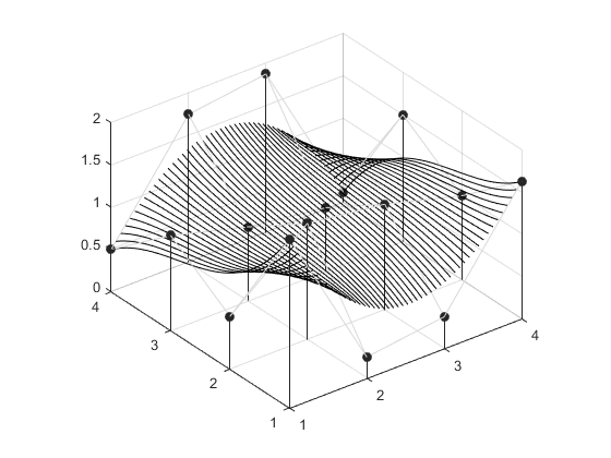
First we'll draw them using stem3.
p = stem3(px,py,pz,'filled');
daspect([1 1 1])
ax = gca;
ax.XTick = 1:4;
ax.YTick = 1:4;
color = [.15 .15 .15];
p.Color = color;
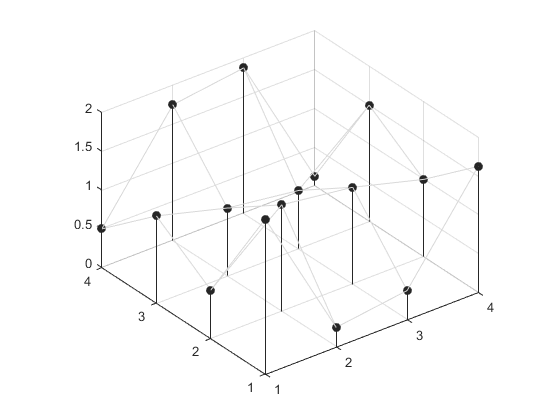
We can connect them into their 4x4 grid by using a surface with FaceColor='none'.
hold on
cpts = surf(px,py,pz);
cpts.FaceColor = 'none';
cpts.EdgeColor = [.85 .85 .85];
Now we're ready to create some patches. All of the patches take the same form. A pair of parameter values u & v yield a point when they're substituted into the following equation.
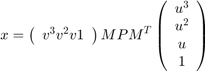
In this equation, the matrix P is our 4x4 matrix of control points, and the matrix M is called the "basis matrix" of the patch. The memo covers several different basis matrices, starting with our old favorite, the cubic Bézier patch. This is the patch that we saw in my first blog post here when we were looking at Newell's teapot. You'll also notice the similarities to the equation for the cubic Bézier curve we saw in my second post.
Mbezier = [-1  3 -3 1; ...
            3 -6  3 0; ...
           -3  3  0 0; ...
            1  0  0 0];
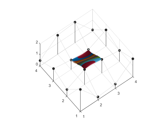
We can use that to generate a surface with one set of isoparameter lines like this:
M = Mbezier;

% U & V vectors
u = linspace(0,1,50);
v = linspace(0,1,50)';
u_powers = [u.^3; u.^2; u; ones(size(u))];
v_powers = [v.^3, v.^2, v, ones(size(v))];

% Multiply to get X,Y, & Z
xout = v_powers * M * px * M' * u_powers;
yout = v_powers * M * py * M' * u_powers;
zout = v_powers * M * pz * M' * u_powers;

% Draw as a surface
hold on
s = surf(xout,yout,zout);
s.FaceColor = 'none';
s.MeshStyle = 'row';
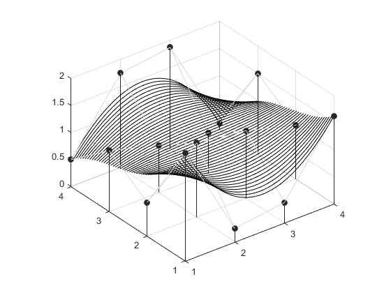
And then the show the other set of isoparameter lines like this:
s.MeshStyle = 'column';
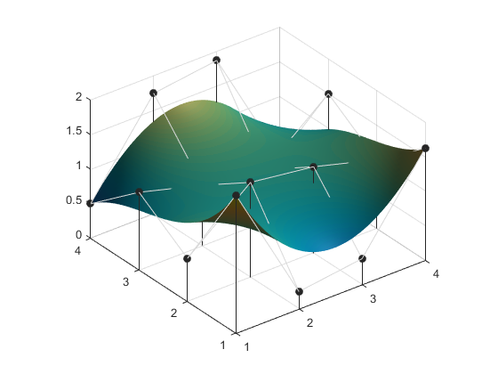
or as a shaded surface with lighting.
s.EdgeColor = 'none';
s.FaceColor = 'interp';
s.FaceLighting = 'gouraud';
s.SpecularStrength = 5/8;
light('Position',[9 -5 8])
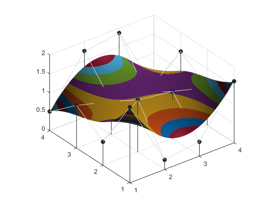
A coarser colormap will add "waterlevel" lines.
colormap(lines(20))
Notice that the Bézier patch has the same characteristics we saw in the earlier blog post about the curves. It passes through the 4 control points in the corners of the 4x4 set, it's tangent to the control point mesh at those corners, and it's completely contained within the bounds of the control point mesh. These are really useful properties and they make Bézier very easy to work with.
The "Patch Work" memo includes the basis matrices for a number of other types of patches, but some of them are a little trickier to work with.
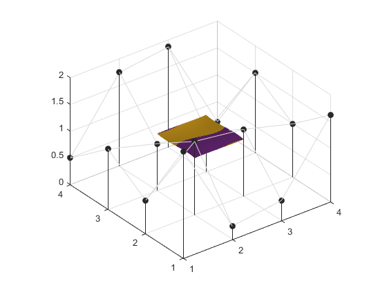
Let's try the Catmull-Rom patch.
Mcatmullrom = [-1  3 -3  1; ...
                2 -5  4 -1; ...
               -1  0  1  0; ...
                0  2  0  0] / 2;
M = Mcatmullrom;
s.XData = v_powers * M * px * M' * u_powers;
s.YData = v_powers * M * py * M' * u_powers;
s.ZData = v_powers * M * pz * M' * u_powers;
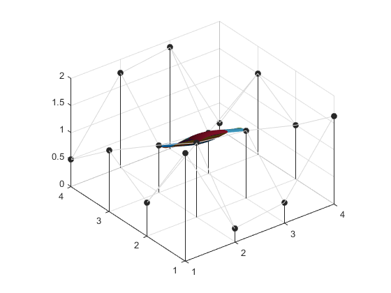
It's a little hard to see from that viewing angle, but the way a Catmull-Rom spline works is that it connects the inner 2x2 points of our control point mesh.
view(-37.5,60)
The other points in the control mesh of a Catmull-Rom patch simply control the tangents at the edges of the patch. The way you usually use these is to have two rows of control points be shared between neighboring patches. This ensures that the patches have a nice, smooth blend where they meet. It is possible to get the same effect with Bézier patches, but it is a little bit trickier.
The basis matrix for the B-spline patch looks like this.
Mbspline = [-1  3 -3 1; ...
             3 -6  3 0; ...
            -3  0  3 0; ...
             1  4  1 0] / 6;
M = Mbspline;
s.XData = v_powers * M * px * M' * u_powers;
s.YData = v_powers * M * py * M' * u_powers;
s.ZData = v_powers * M * pz * M' * u_powers;
view(3)
You can see that this patch also only covers the inner 2x2 of our control point mesh, and it doesn't even pass through those points. This property makes the B-spline patch kind of challenging to work with when you're trying to model something.
But the "patch work" memo also shows how to convert the control points of one kind of patch to those of another kind of patch. To do this, we need what it calls "to-from" matrices. We can use this to convert our friendly Bézier patch control points into ones which work for the B-spline patch by using this matrix.
Mtofrom = [6 -7  2 0; ...
           0  2 -1 0; ...
           0 -1  2 0; ...
           0  2 -7 6];

pxnew = Mtofrom * px * Mtofrom';
pynew = Mtofrom * py * Mtofrom';
pznew = Mtofrom * pz * Mtofrom';
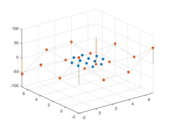
If we compare the control points before and after this transformation, we can see that the ones for the B-spline patch extand way outside the ones for the Bézier patch, and the Z range is much wider.
f2 = figure;
p1 = stem3(px,py,pz,'filled');
hold on
p2 = stem3(pxnew,pynew,pznew,'filled');
surf(pxnew,pynew,pznew,'FaceColor','none','EdgeColor',[.85 .85 .85])
xlim([-inf inf])
ylim([-inf inf])
But when we use these new points with the basis matrix for the B-spline patch, they will give us the same surface we got with the Bézier patch using the original control points.
delete(f2)
s.XData = v_powers * M * pxnew * M' * u_powers;
s.YData = v_powers * M * pynew * M' * u_powers;
s.ZData = v_powers * M * pznew * M' * u_powers;

Being able to convert between different patch types is extremely useful because the different types have different properties which are useful in different situations.
You can find all of the to-from matrices in this file.
But there are more goodies hiding in this memo. We saw when we talked about parametric curves that being able to compute partial derivatives of the curves is very useful for creating tangents and normals. The same is true when you're working with surface patches, and this memo has a section on how to compute partial derivatives of the patches. To compute those, we need the following two matrices.
du = [0 3 0 0; ...
      0 0 2 0; ...
      0 0 0 1; ...
      0 0 0 0];

dv = [0 0 0 0; ...
      3 0 0 0; ...
      0 2 0 0; ...
      0 0 1 0];
We'll create a low-res parameterization.
M = Mbezier;
u = linspace(0,1,10);
v = linspace(0,1,10)';
u_powers = [u.^3; u.^2; u; ones(size(u))];
v_powers = [v.^3, v.^2, v, ones(size(v))];

xout = v_powers * M * px * M' * u_powers;
yout = v_powers * M * py * M' * u_powers;
zout = v_powers * M * pz * M' * u_powers;
And then we use the matrices du and dv like this:
dxdu = v_powers * M * px * M' * du * u_powers;
dydu = v_powers * M * py * M' * du * u_powers;
dzdu = v_powers * M * pz * M' * du * u_powers;
dxdv = v_powers * dv * M * px * M' * u_powers;
dydv = v_powers * dv * M * py * M' * u_powers;
dzdv = v_powers * dv * M * pz * M' * u_powers;
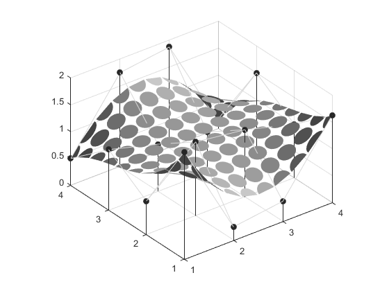
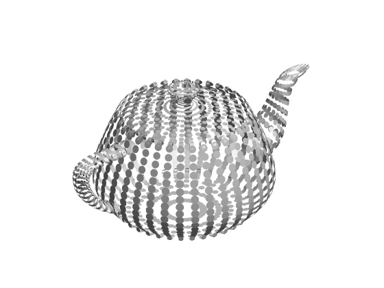
We could use the cross product of those two vectors to compute normals which are much smoother than what the surface command can create. Or we can use them directly to cover the surface with a bunch of tangent circles like this:
xlim manual
ylim manual
zlim manual
delete(s)
radius = .05;
theta = linspace(0,2*pi,72); % points around the circles
for i=1:numel(xout)
    % c + r*(cos(theta)*dp/du + sin(theta)*dp/dv)
    cx = xout(i) + radius*(cos(theta)*dxdu(i) + sin(theta)*dxdv(i));
    cy = yout(i) + radius*(cos(theta)*dydu(i) + sin(theta)*dydv(i));
    cz = zout(i) + radius*(cos(theta)*dzdu(i) + sin(theta)*dzdv(i));
    h = patch(cx,cy,cz,zeros(size(cx)));
    h.FaceColor = [.875 .875 .875];
    h.EdgeColor = 'none';
end
Can you combine this with what we did in the teapot blog post to create a picture that looks like this?
- Category:
- Geometry

