
Tie a Ribbon Round It (Parametric Curves Part 1)
Tie a Ribbon Round It (Parametric Curves: Part 1)
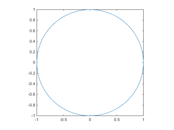
Parametric curves are easy to draw in MATLAB. For example, we can use the parametric equation for a circle like so:


t = linspace(0,2*pi,128);
x = cos(t);
y = sin(t);

plot(x,y);
axis square
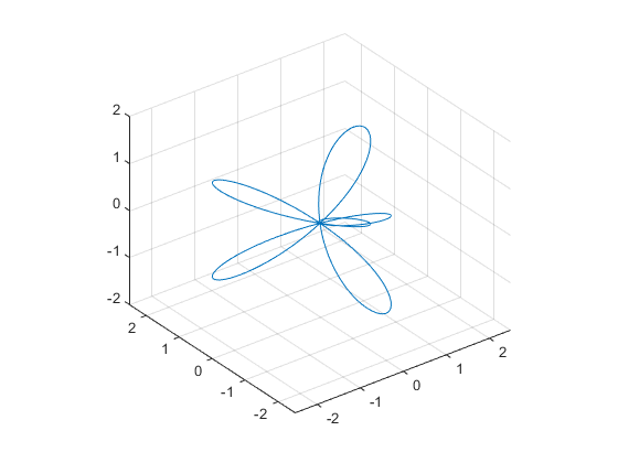
The same thing works in 3D.


t = linspace(0,2*pi,256);
x = 3*cos(t)+cos(10*t).*cos(t);
y = 3*sin(t)+cos(10*t).*sin(t);
z = sin(10*t);

plot3(x,y,z);
ax = gca;
ax.DataAspectRatio = [1 1 1];
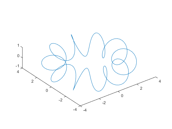
But it can be tough to see what the curve is doing in 3D when you draw it as a line. It can be a lot clearer if we sweep a surface along the curve. To do that, we just need to find a series of vectors which are normal to the curve at each point. We can do that pretty easily if we remember our partial derivatives. If we take the first derivative of the points on the curve with respect to  .
.

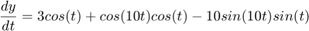
dxdt = -3*sin(t) - cos(10*t).*sin(t) - 10*sin(10*t).*cos(t);
dydt = 3*cos(t) + cos(10*t).*cos(t) - 10*sin(10*t).*sin(t);
dzdt = 10*cos(10*t);
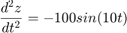
We'll get a set of tangent vectors, but the magnitudes will be a little strange. The magnitude is actually the velocity of the curve at that point. We can normalize the tangent vectors using the following function.
function [xo, yo, zo,l] = normalize_vector(xi,yi,zi)
  l=sqrt(xi.^2+yi.^2+zi.^2);
  l(l~=0) = 1./l(l~=0);
  xo = xi.*l;
  yo = yi.*l;
  zo = zi.*l;
Like this:
[tx,ty,tz] = normalize_vector(dxdt,dydt,dzdt);
And then we can plot them along with the curve using this function.
function plot_vectors(px,py,pz, vx,vy,vz)
% Plot the curve [x,y,z] and the vectors [vx,vy,vz]
  % First the curve
  plot3(px,py,pz);
  hold on
  % Then the vectors
  lx = [px; px+vx; nan(size(px))];
  ly = [py; py+vy; nan(size(py))];
  lz = [pz; pz+vz; nan(size(pz))];
  plot3(lx(:),ly(:),lz(:));
  % Finally add markers at the "heads"
  plot3(px+vx,py+vy,pz+vz,'.');
  grid on
  hold off
plot_vectors(x,y,z, tx,ty,tz);
ax.DataAspectRatio = [1 1 1];
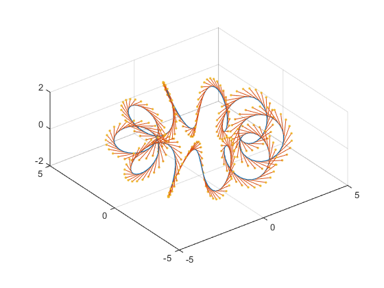
But we need a vector which is normal to the curve, not one which is tangent to it. We need to keep going. The second partial with respect to $t$ actually does what we want.


d2xdt2 = -3*cos(t) + 20*sin(10*t).*sin(t) - 101*cos(10*t).*cos(t);
d2ydt2 = -3*sin(t) - 101*cos(10*t).*sin(t) - 20*sin(10*t).*cos(t);
d2zdt2 = -100*sin(10*t);
If we plot those vectors, we can see that they all point towards the circle that our curve is orbiting around.
[nx,ny,nz] = normalize_vector(d2xdt2,d2ydt2,d2zdt2);
plot_vectors(x,y,z, nx,ny,nz);
ax.DataAspectRatio = [1 1 1];
That gives us everything we need to create a ribbon. We simply turn the 1xN array of points into a 2xN array of points by adding and subtracting half of normal vectors from the points.
sx = [x+nx/2; x-nx/2];
sy = [y+ny/2; y-ny/2];
sz = [z+nz/2; z-nz/2];
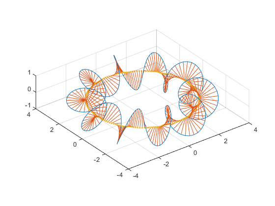
We can give that 2xN array to surf to create a long, thin surface which is the ribbon.
I'll use the hsv colormap because it's cyclic, just like our curve.
h = surf(sx,sy,sz,[t;t]);
ax.DataAspectRatio = [1 1 1];
colormap(hsv(256))
This lets us clearly see how the curve moves through three dimensions. We can also turn on a light to see more detail, and turn off the edges to make it a little prettier.
h.EdgeColor = 'none';
h.FaceColor = 'interp';
h.FaceLighting = 'gouraud';
camlight headlight
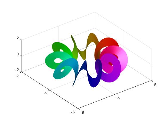
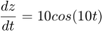
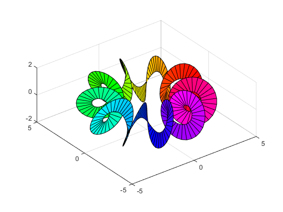
Next time we'll look at more things we can do with this technique. In the meantime, can you use these equations:
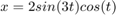

to get something that looks like this?
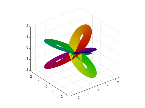
It's a little easier to understand than this wireframe view, isn't it?
- Category:
- Geometry

