
Fill Between
Fill Between
One question I'm often asked is how to fill the area between two plotted curves. It is possible to do this, but it involves some details which aren't obvious, so let's walk through what's involved.
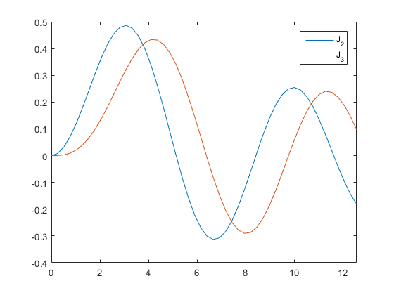
First we need a simple example. I'm going to plot these two Bessel functions.
x = linspace(0,8,50);
y1 = besselj(2,x);
y2 = besselj(3,x);
plot(x,y1)
hold on
plot(x,y2)
hold off
legend('J_2','J_3')
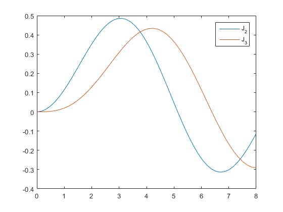
I want to highlight all of the areas where the value of 3rd Bessel function is larger than the value of the 2nd. In other words, I want to fill the area above the blue curve and below the red curve.
To fill an area, we're going to want to use the fill function. This function takes three arguments: X, Y, and Color. We can get these from our data by building a mask of the locations where y2 > y1. Our Y values are going to be the Y's from each of the two curves at the locations in that mask. And we'll need two copies of the X. We also need to flip the second half because fill is going to go left to right along the bottom, and right to left along the top.
mask = y2 > y1;
fx = [x(mask), fliplr(x(mask))];
fy = [y1(mask), fliplr(y2(mask))];
hold on
fill_color = [.929 .694 .125];
fh = fill(fx,fy,fill_color);
hold off
That's a start, but we can see some issues. The fill is drawing a black line over the curves. We can get rid of that by setting its EdgeColor to none.
fh.EdgeColor = 'none';

But that still doesn't look right. What's happening is that the fill is on top of the curves. We can see that more clearly if we make our lines wider.
set(findobj(gca,'Type','line'),'LineWidth',3);
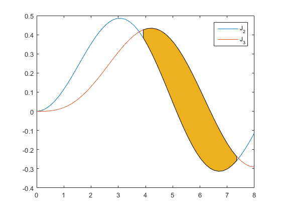
To fix that, we need to move it to the back. We can do that with the uistack function.
uistack(fh,'bottom')

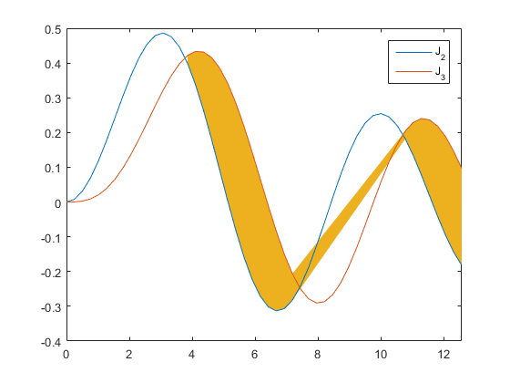
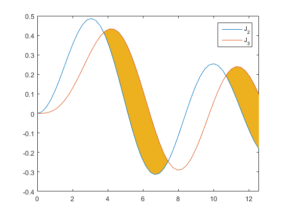
But we still have some work to do. Look at the little missing piece between X=3 and X=4. And it looks even worse if we zoom out.
cla
x = linspace(0,4*pi,50);
y1 = besselj(2,x);
y2 = besselj(3,x);
plot(x,y1)
hold on
plot(x,y2)
legend('J_2','J_3')
xlim([0 inf])

mask = y2 > y1;
fx = [x(mask), fliplr(x(mask))];
fy = [y1(mask), fliplr(y2(mask))];
fill_color = [.929 .694 .125];
fh = fill(fx,fy,fill_color);
fh.EdgeColor = 'none';
uistack(fh,'bottom')
hold off
These two problems are happening because the two curves cross in between values in our data. We need to do interpolation to find the point where they cross and add that intersection point to the fill. They intersect at X=3.7689, but the nearest x value we have in the plot is 3.8468. This means that we need to do interpolation between the data values to figure out exactly where the lines cross so that we can put an accurate end on our filled area.
Let's get rid of that fill, and create a pair of helper functions for doing linear interpolation.
delete(fh)

hold on
output = [];
% Calculate t in range [0 1]
calct = @(n) (n(3,1)-n(2,1))/(n(3,1)-n(2,1)-n(3,2)+n(2,2));
% Generate interpolated X and Y values
interp = @(t,n) n(:,1) + t*(n(:,2) - n(:,1));
Now we loop over the values and copy the ones where y2 > y1. But as we do that, we look for the places where the lines cross. When we find one, we do linear interpolation to find the crossing point, and we add that to the points we're saving. The result looks like this:
for i=1:length(x)
    % If y2 is below y1, then we don't need to add this point.
	if y2(i) <= y1(i)
        % But first, if that wasn't true for the previous point, then add the
        % crossing.
        if i>1 && y2(i-1) > y1(i-1)
            neighborhood = [x(i-1), x(i); y1(i-1), y1(i); y2(i-1), y2(i)];
            t = calct(neighborhood);
            output(:,end+1) = interp(t,neighborhood);
        end
    else
    % Otherwise y2 is above y1, and we do need to add this point. But first
    % ...
        % ... if that wasn't true for the previous point, then add the
        % crossing.
        if i>1 && y2(i-1) <= y1(i-1)
            neighborhood = [x(i-1), x(i); y1(i-1), y1(i); y2(i-1), y2(i)];
            t = calct(neighborhood);
            output(:,end+1) = interp(t,neighborhood);
        end

        % add this point.
        output(:,end+1) = [x(i); y2(i); y1(i)];
    end
end
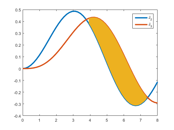
At this point we have an X array and two Y arrays (one for the top and one for the bottom), just like we did before. But they have those crossing points inserted in the correct places.
xout = output(1,:);
topout = output(2,:);
botout = output(3,:);
fh = fill([xout fliplr(xout)],[botout fliplr(topout)],fill_color);
fh.EdgeColor = 'none';
uistack(fh,'bottom')
hold off
That looks much better.
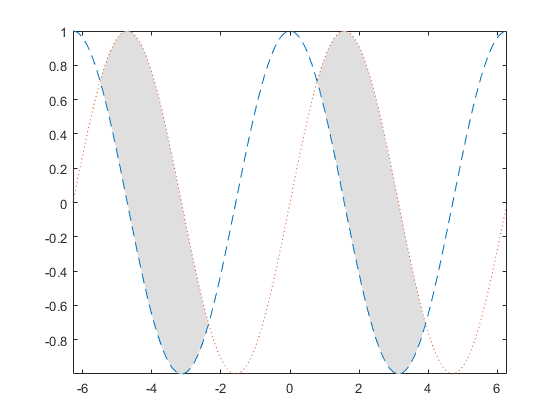
We can easily put that into a function that we can reuse with other plots, like this one:
theta = linspace(-2*pi,2*pi,150);
c = cos(theta);
s = sin(theta);
plot(theta,c,'--')
hold on
plot(theta,s,':')
hf = fill_between(theta,c,s);
hf.FaceColor = [.875 .875 .875];
axis tight
hold off
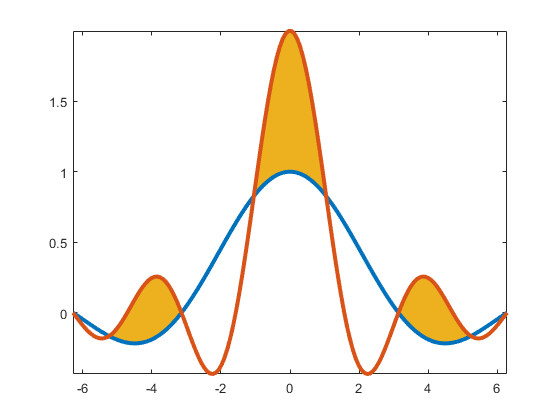
... or this one:
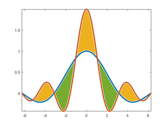
y1 = sin(theta)  ./ theta;
y2 = sin(2*theta) ./ theta;
hl = plot(theta,[y1; y2]);
hf = fill_between(theta,y1,y2);
set(hl,'LineWidth',3)
axis tight
You can even switch the inputs to color the other regions.
hf(2) = fill_between(theta,y2,y1);
hf(2).FaceColor = [.466 .674 .188];

But maybe a bit of a white border between the curves and the fills would make it look nicer.
htmp = [copyobj(hl(1),gca), copyobj(hl(2),gca)];
set(htmp,'LineWidth',5,'Color','white')
uistack(htmp,'down')
uistack(htmp,'down')
Once you know the basic idea, you can probably extend this to do lots of other interesting tricks.
- 범주:
- Charts

