Signed Distance Fields
Recently I heard from a MATLAB user who was trying to draw tubes along a curve using this blog post I wrote a while back. Unfortunately her curve was a bit more complex than the ones I used in that post. That approach of sweeping a 2D shape along a curve has a number of interesting edge cases that you'll encounter when your curves are complex.
In particular, her curve actually had a "fork" in it. This is a particularly tough case for the sweep approach. You basically need to sweep each of the two halves of the fork, and then slice off the parts of one sweep that are inside the other one. The math for this gets rather tricky.
Luckily there's another approach to this problem. This one is fairly compute intensive, but it's quite a bit simpler to implement. It's called signed distance fields. Let's take a look at how you would solve this problem using an SDF.
First we'll need some sample data. Here's one I made. I have 4 vertices.
verts = [-1    0 0; ...
        1/2    0 0; ...
          2  3/4 0; ...
          2 -3/4 0];
radius = .5;
And I have 3 line segments which connect the four vertices.
segments = [1 2; 2 3; 2 4];
Let's draw the segments.
for i=1:size(segments,1)
    line(verts(segments(i,:),1),verts(segments(i,:),2),verts(segments(i,:),3))
end
box on
daspect([1 1 1])
view(3)
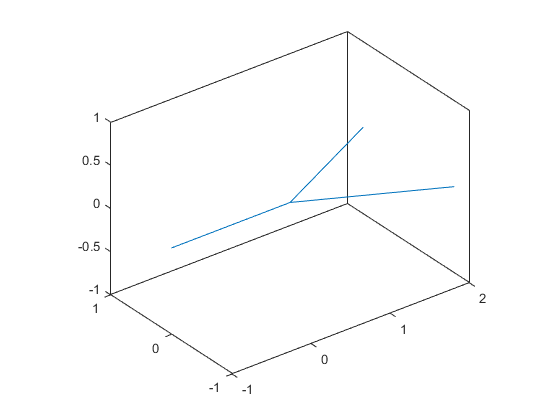
So we want a tube-like surface which follows those line segments, and smoothly blends between two which fork off to the right.
The first thing we'll do is build a 3D grid over the space we're interested in. The bigger you make the grid, the better your surface will be, but the amount of memory you’re using will climb quickly.
[y,x,z] = ndgrid(linspace(-1.25,1.25,90),linspace(-1,2.25,90),linspace(-0.75,0.75,45));
And now we'll create a 4th array to hold our signed distance field.
d = zeros(size(z));
Now we loop over all of the grid points. At each point in the grid, we'll loop over all of the line segments and calculate the distance from the grid point to the closest point on the line segment. We'll keep the smallest distance and save it in d.
for i=1:numel(z)
    p = [x(i),y(i),z(i)];

    % Intialize our distance to inf.
    closest = inf;

    % Loop over all of the line segments.
    for j=1:size(segments,1)
        q1 = verts(segments(j,1),:);
        q2 = verts(segments(j,2),:);

        % For line segment q1 + t*(q2-q1), compute the value of t where
        % distance to p is minimized. Clamp to [0 1] so we don't go off
        % the end of the line segment.
        invlen2 = 1/dot(q2-q1,q2-q1);
        t = max(0,min(1,-dot(q1-p,q2-q1)*invlen2));
        v = q1 + t*(q2-q1);

        % Is that  the smallest we've seen for this grid element?
        closest = min(closest, norm(v-p)-radius);
    end

    % Insert the distance into the array.
    d(i) = closest;
end
Notice that the value I saved into the array d was the distance from that grid point to a line segment, minus the radius of the surface at that point on the line segment. That means that anywhere in our grid that d is less than 0 is inside the tube, and anywhere that d is greater than 0 is outside the tube. As we saw in this post about implicit surfaces, this is a job for the isosurface function.
isosurface(x,y,z,d,0)
camlight
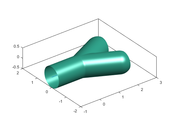
And we can see that this surface lines up nicely with our original model, and does a nice job of blending that fork.
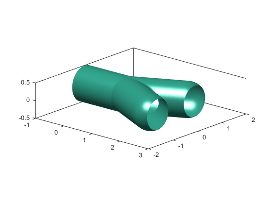
Let's delete the lines and change the view so we can see inside the fork. See how tidy that intersection is? That would be hard to do with the other approach.
Also notice how it rounds off the ends. We can see inside because I made the grid pretty tight. If my grid had been a bit larger, then each of the three ends would be capped by a hemisphere. This is characteristic of the signed distance fields approach.
delete(findobj(gca,'Type','line'))
view([41 18])
But what if we had a different radius at each vertex, and wanted the tube to interpolate between the radii at the end of each segment?
Let's say that we wanted the following radii at each vertex.
radii = [.5 .45 .125 .25];

cla
for i=1:size(segments,1)
    line(verts(segments(i,:),1),verts(segments(i,:),2),verts(segments(i,:),3))
end
[xs,ys,zs] = sphere;
for i=1:size(verts,1)
    surface(verts(i,1)+radii(i)*xs, ...
            verts(i,2)+radii(i)*ys, ...
            verts(i,3)+radii(i)*zs, ...
        'FaceColor','yellow','EdgeColor','none');
end
camlight
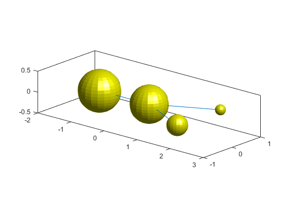
This is a little trickier, but it's basically just a matter of changing our distance function. We can no longer use the simple formula for the distance between a point and the centerline.
I found a distance function that will do the job in this paper:
| Fast distance computation between a point and cylinders, cones, line swept spheres and cone-spheres |
| Aurelien Barbier and Eric Galin |
| LIRIS - CNRS |
| Universite Claude Bernard Lyon 1 |
| 69622 Villeurbanne Cedex, France |
The authors call this primitive with a centerline and a radius at each end the "cone-sphere" primitive.
This distance equation is more complex, so I'll precompute some terms to help with performance.
nsegments = size(segments,1);
invlen2 = zeros(1,nsegments);
trange = zeros(nsegments,2);
adj_radii = zeros(nsegments,2);
for i=1:nsegments
    q1 = verts(segments(i,1),:);
    q2 = verts(segments(i,2),:);
    len2 = dot(q2-q1,q2-q1);
    invlen2(i) = 1/len2;

    r1 = radii(segments(i,1));
    r2 = radii(segments(i,2));
    delta = r1-r2;
    s = sqrt(len2 - delta^2);

    dl = delta * invlen2(i);
    sl = s * sqrt(invlen2(i));

    trange(i,1) = r1 * dl;
    trange(i,2) = 1 + r2 * dl;
    adj_radii(i,1) = r1 * sl;
    adj_radii(i,2) = r2 * sl;
end
Now we can repeat our loop with this new distance formula.
for i=1:numel(z)
    p = [x(i),y(i),z(i)];

    closest = inf;
    for j=1:size(segments,1)
        q1 = verts(segments(j,1),:);
        q2 = verts(segments(j,2),:);
        r1 = radii(segments(j,1));
        r2 = radii(segments(j,2));

        t = -dot(q1-p,q2-q1)*invlen2(j);
        if t<trange(j,1)
            v = q1;
            r = r1;
        elseif t>trange(j,2)
            v = q2;
            r = r2;
        else
            v = q1 + t*(q2-q1);
            adj_t = (t-trange(j,1)) / (trange(j,2)-trange(j,1));
            r = adj_radii(j,1) + adj_t*(adj_radii(j,2)-adj_radii(j,1));
        end

        closest = min(closest, norm(v-p)-r);
    end

    d(i) = closest;
end
And then we can use isosurface, just like we did before.
isosurface(x,y,z,d,0)
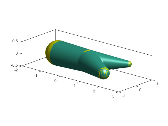
See how the surface lines up with the spheres? Now we'll delete them to get a better look.
delete(findobj(gca,'Type','line'))
delete(findobj(gca,'Type','surface'))
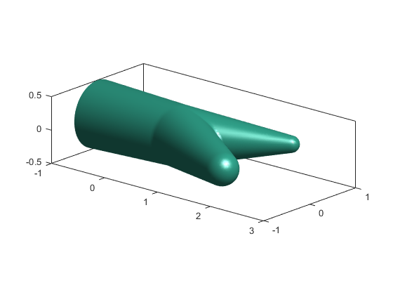
Here's another isosurface I made from these 6 edges of a tetrahedron using this technique.
verts = randn(4,3);
segments = nchoosek(1:4,2);
radii = 5/8 * rand(1,4);

That took quite a while to compute, but it would have been awful tricky to draw it with the sweep approach.
Whenever you want to wrap a surface around a complex shape, then signed distance functions are a technique that you should consider.
- Category:
- Geometry


