On the Grid

One type of question that I'm often asked is about how to use various visualization techniques with what is sometimes called "scatter data". This is data that is a list of individual measurements. These measurements often have locations associated with them, but that's not enough for many visualization techniques. These techniques also want grid information. This is information about how the measurements connect to each other. Let's take a look at a couple of ways in which we can get this grid information.

First we'll need some example data. Here I have 250 measurements. Each one has a 2D location and a value.

npts = 250;
rng default
x = 2*randn(npts,1);
y = 2*randn(npts,1);
v = sin(x) .* sin(y);

Scatter data, which is sometimes known as column data, gets its name from the fact that the scatter plot is the one visualization technique which is really designed for this type of data.

scatter(x,y,36,v,'filled')
colorbar
xlim([-2*pi 2*pi])
ylim([-2*pi 2*pi])

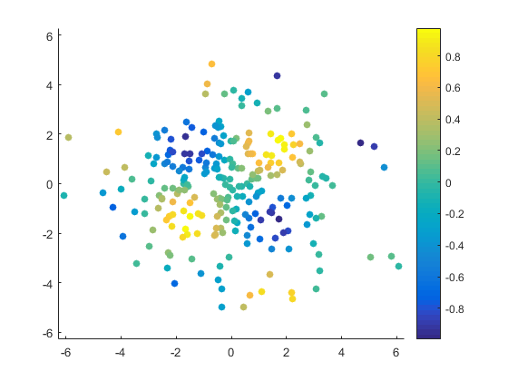
You can sort of see the pattern of v in that picture. If you squint hard enough. But it'd be a lot nicer if we had colors in between the dots. The pcolor function can draw that kind of picture, but it needs a particular type of input known as a "structured grid". We can create this type of grid by using the meshgrid function.

[xg,yg] = meshgrid(linspace(-2*pi,2*pi,125));
size(xg)
size(yg)

ans =

   125   125


ans =

   125   125

But that's just the grid. That's not enough. We also need to get our values onto the grid. One good way to do this is with scatteredInterpolant.

F = scatteredInterpolant(x,y,v);
vg = F(xg,yg);
h = pcolor(xg,yg,vg);

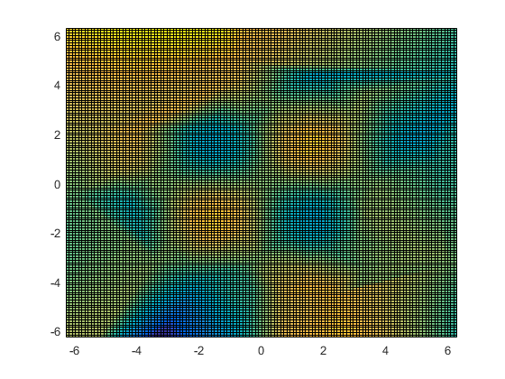
We don't really want to see the grid here, so I'll turn it off.

h.EdgeColor = 'none';

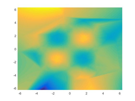
And add a colorbar so we can see what values we're getting.

colorbar

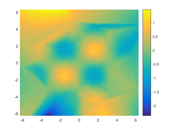
That looks pretty good, but not great. For one thing, the range of values is way too large. We can't possibly have sin(x)*sin(y) reaching values less than -2, can we?

caxis([-1 1])

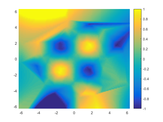
And while the middle of the picture is pretty good, look at that big yellow blob in the upper left and the big blue blob on the bottom. Where did those come from?

Both of these issues are because out at the edges of the grid scatteredInterpolant is extrapolating past the values we gave it, rather than interpolating between them. Extrapolation is almost always a fairly dicey operation. To do it successfully, you really need to know a lot about the data you're working with, and use a lot of care in choosing your extrapolation function.

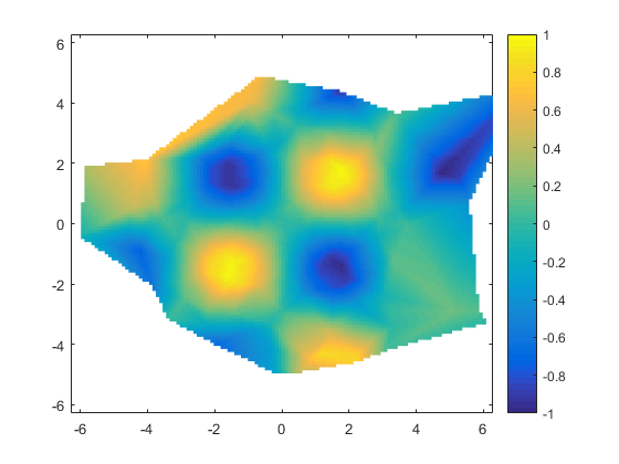
Often it's better to just discard the parts of the grid which require extrapolation. That's actually pretty easy to do. We just need to insert nans into the values at those points on the grid. We can find those points on the grid by using convhull and inpolygon.

p = convhull(x,y);
xp = x(p);
yp = y(p);
inmask = inpolygon(xg(:),yg(:), xp,yp);
vg(~inmask) = nan;
h = pcolor(xg,yg,vg);
h.EdgeColor = 'none';
xlim([-2*pi 2*pi])
ylim([-2*pi 2*pi])
caxis([-1 1])
colorbar

I could use either the boundary function or the alphaShape function instead of convhull here.

As you can see, boundary will be more aggressive about removing portions of the grid which are far away from any sample points. It also has a parameter which lets you adjust that.

b = boundary(x,y);
inmask = inpolygon(xg(:),yg(:), x(b),y(b));

vg = F(xg,yg);
vg(~inmask) = nan;
h = pcolor(xg,yg,vg);
h.EdgeColor = 'none';
xlim([-2*pi 2*pi])
ylim([-2*pi 2*pi])
caxis([-1 1])
colorbar

Another thing that is very important when you're gridding scatter data is choosing the right grid resolution. The scatteredInterpolant is going to work best when the resolution of the grid is close to the spacing of your original sample points. A grid that's too fine usually isn't a big problem (except for the amount of memory you consume), but if your grid is much coarser than the spacing of the input points, then you may see aliasing artifacts. That's because the scatteredInterpolant doesn't really low-pass filter for you. This issue can become quite challenging when the spacing between your sample points varies widely. A good grid resolution for one area of your data might not be appropriate for another area.

But the "structured grid" isn't the only type of grid available to us. There's also what's known as an "unstructured grid". In a structured grid, we just lay out the values in a 2D array, and know that each one is connected to its immediate neighbors. In an unstructured mesh, we'll keep our columns of data values, and add an extra variable that lists how they're connected.

BTW, I've always thought this naming convention was a little silly because the whole point of an unstructured grid is that you have to spell out the structure in detail. The word "unstructured" doesn't seem like a good description of that.

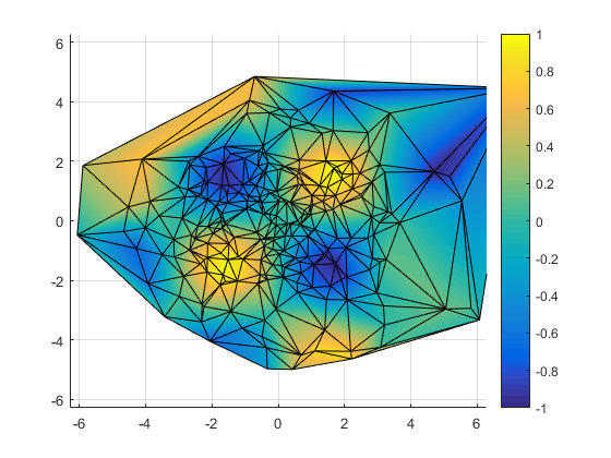
The simplest type of unstructured grid is a "triangle mesh". In a triangle mesh, we have Nx3 array which is a list of triangles which each connect three of the original points. One easy way to create a triangle mesh is to use the delaunayTriangulation function.

dt = delaunayTriangulation(x,y);

Once we have our triangle mesh, we can draw it using the trisurf function.

h = trisurf(dt.ConnectivityList,x,y,zeros(npts,1),v);
h.FaceColor = 'interp';
view(2)
xlim([-2*pi 2*pi])
ylim([-2*pi 2*pi])
caxis([-1 1])
colorbar

Again, I'll hide the grid.

h.EdgeColor = 'none';

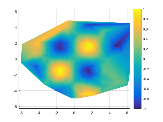
There are some advantages to each of these two approaches.

The triangle mesh is nice and compact, and it often has fewer gridding artifacts. In particular, it naturally handles that case where the spacing between the points varies a lot by placing more triangles where the data is sampled more finely.

On the other hand, MATLAB has more visualization techniques which work on a structured grid. For example, I could use one of the contour functions on the structured grid, but MATLAB doesn't come with a contour function that will work on triangle meshes, although you can find some on the File Exchange.

These two examples are just an introduction to the powerful tools that MATLAB provides for gridding scatter data. If you find one of them useful, you might want to explore the different options that scatteredInterpolant accepts, and some of the other functions that are available. And you might also want to start a conversation on MATLAB Answers. There are a number of people there who have experience with gridding different types of data.

Get the MATLAB code

Published with MATLAB® R2015b