
The new solution framework for Ordinary Differential Equations (ODEs) in MATLAB R2023b
Along with linear algebra, one of the iconic features of MATLAB in my mind is how it handles ordinary differential equations (ODEs). ODEs have been part of MATLAB almost since the very beginning.
One of the features of how MATLAB traditionally allows users to solve ODEs is that it provides a suite of functions. For many years, there were 7 routines in the MATLAB suite, described in this 2014 post by Cleve Moler and in more detail in the 1997 paper, The MATLAB ODE Suite. In 2021b, 2 new high-order methods were added to the suite, ode78 and ode89 based on the algorithms described in the paper Numerically optimal Runge–Kutta pairs with interpolants.
The design of the suite was elegant and has served the community well for over 25 years! However, MATLAB has evolved a lot since it was designed and user-expectations have evolved with it. It was felt that it was time for a fresh look at how to solve ODEs in MATLAB, one that would additionally support our future plans in a modern and elegant manner.
Before I dive into the new interface, I'd like to make it clear that the existing suite of ODE functions are not going anywhere! Millions of lines of code make use of ode45 and friends and we have no plans on doing anything that would break that code. This is about adding functionality, not taking anything away.
Furthermore, the focus of this release is the new interface. There are no new solvers or any fundamentally new functionality....yet! However, some things will be significantly easier to do using the new interface.
With that said, let's take a look at how the new design looks.
Solving ODEs in MATLAB the OOP way
Say we want to solve the ODE
with the initial condition over the interval
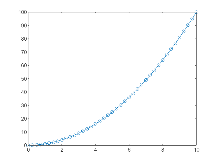
With the new interface, we can set up and solve this problem as follows
F = ode(ODEFcn=@(t,y) 2*t,InitialTime=0,InitialValue=0); % Set up the problem by creating an ode object
sol = solve(F,0,10); % Solve it over the interval [0,10]
plot(sol.Time,sol.Solution,"-o") % Plot the solution
An alternative way to proceed would have been to start with an empty ode object and add one property at a time:
F = ode; % Empty ode object called F
F.ODEFcn = @(t,y) 2*t; % Add the function we want to solve to F
F.InitialTime = 0; % Add the initial time to F
F.InitialValue = 0; % Add the initial value to F
Once our problem is set up, we pass it to the solve function.
sol = solve(F,0,10);
sol
You access either property with . notation
sol.Solution
sol.Time
Automatic solver selection
One of the first things to note in the above workflow is that we didn't choose a solver. That is, I didn't have to think about if I should use ode45, ode78 etc. All I did was state the problem mathematically and ask MATLAB to solve it. Let's take a closer look at the details.
I set up my problem like this:
F = ode(ODEFcn=@(t,y) 2*t,InitialTime=0,InitialValue=0);
F is an ode object:
class(F)
I can see the details by evaluating F
F
The object display separates the mathematical problem definition from how we are going to solve it. By default, the Solver property of the class is set to "auto" which means that MATLAB attempts to choose a suitable solver based on various properties of the problem we've asked it to solve. In this case it has chosen ode45 which is a pretty safe bet for many problems.
Ask for a tighter tolerance for this problem, however, and it switches to using ode78.
F.RelativeTolerance = 1e-7
At this stage, MATLAB hasn't solved anything. We've just set up our problem and made decisions about how we are going to solve it. We need the solve function to complete the job.
One thing to bear in mind is that the solver that "auto" chooses may change in future releases for a number of reasons. For example, we may improve the heuristics used to select the best solver or maybe add new solvers that do a better job for a given problem.
If you want to override what MATLAB chooses and fix the solver type you can do that as follows
F.Solver = "ode45" % Force the framework to use ode45.
Trying a stiff ODE problem
I was curious about how it would handle a stiff ODE and so fed it the example given by Cleve in his blog post Ordinary Differential Equations, Stiffness.
delta = 0.0001;
CleveF = ode(ODEFcn=@(t,y) y^2 - y^3);
CleveF.InitialTime = 0;
CleveF.InitialValue = delta;
sol = solve(CleveF,0,2/delta);
plot(sol.Time,sol.Solution,'-o')
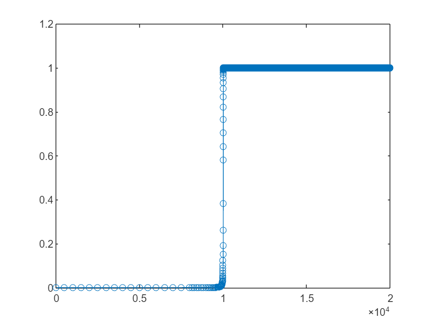
Looks reasonable. Following Cleve's suggestion, we zoom in on the steady state that begins at x=1 and see that the solver is working hard to do its job, just as it did when Cleve explicitly chose ode45.
plot(sol.Time,sol.Solution,'-o')
xlim([10006.3 10112.1])
ylim([0.99615 1.00250])
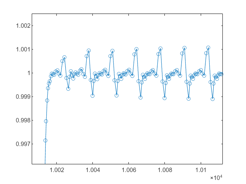
Sure enough, the "auto" option has also chosen ode45 in this case.
CleveF.SelectedSolver
Using the old solver suite, I'd now have to dig into the documentation and read about the stiff solvers available to me before trying those out. With the new interface, however, I just tell it that I think the problem is stiff and it will choose a stiff solver for me.
CleveF.Solver = "stiff"
stiffSol = solve(CleveF,0,2/delta);
plot(stiffSol.Time,stiffSol.Solution,'-o')
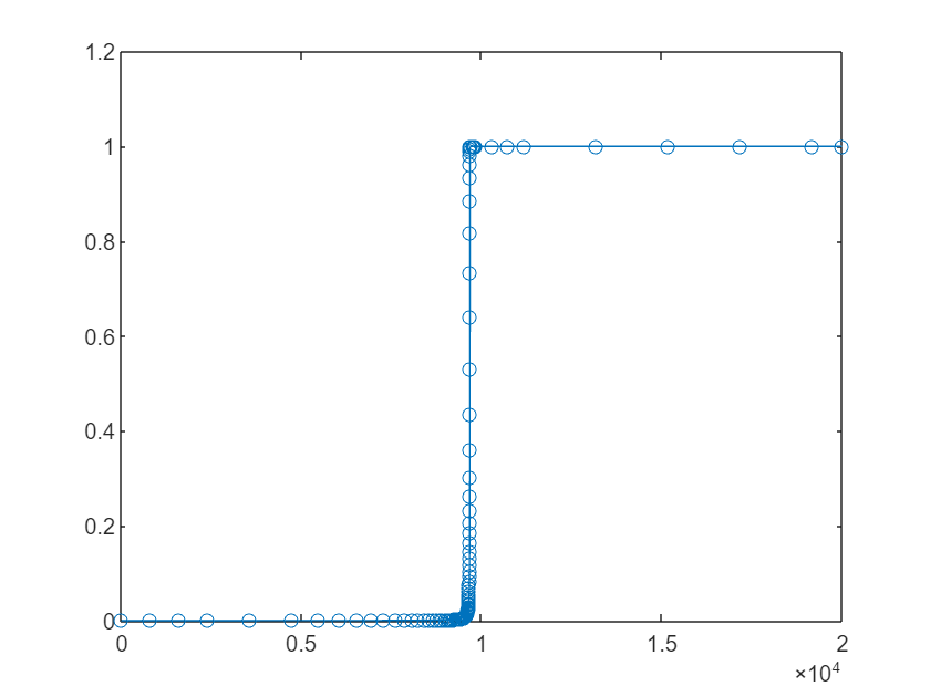
Zooming in at x=1:
plot(stiffSol.Time,stiffSol.Solution,'-o')
xlim([9620.2 9748.2])
ylim([0.99464 1.00232])
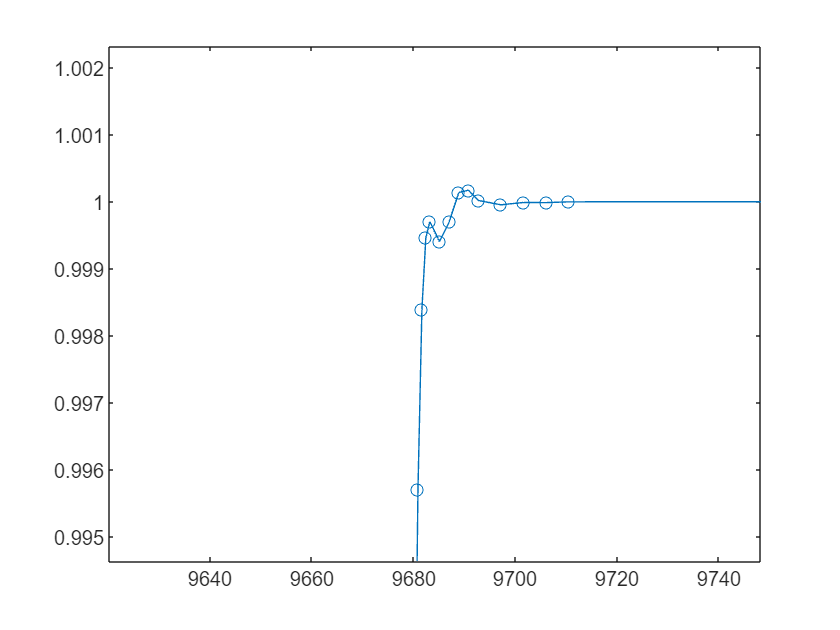
Much better behaved!
Being able to tell MATLAB that the problem is "stiff" makes life a little easier than before but I was a disappointed that "auto" didn't realise that my problem was stiff and choose a relevant solver for me.
I reached out to development to ask why it failed me. They told me that the automatic solver selection is a heuristic that operates without peering inside your equations. It reacts to the data you supply to define the problem, e.g. if you've supplied a Jacobian, what the relative tolerances are, etc. There's no attempt to diagnose stiffness at all. That's why there are "auto", "stiff", and "nonstiff" automatic modes.
Of course, this may change in future releases. Now this feature exists, it will be possible to improve on it and its already pretty useful!
More flexible in time
Consider the following classic system of first-order ODEs that describes simple harmonic motion
$ \frac{dy_1}{dt} = y_2 \ \frac{dy_2}{dt} = -y_1 $
subject to the initial conditions and
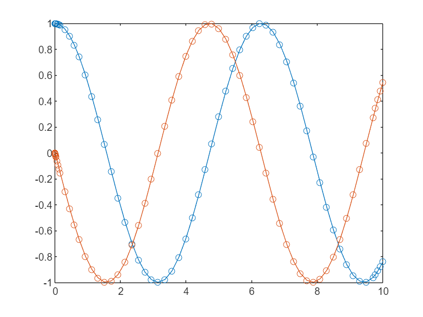
With the classic suite of solvers, you might solve this as follows
y0 = [1; 0]; % initial conditions: y1(0)=1, y2(0)=0
tspan = [0 10]; % time interval from 0 to 10 for the solution
[t,y] = ode45(@(t,y)[y(2);-y(1)], tspan,y0);
plot(t,y,"-o")
So far so simple. Imagine now that I want to go backwards in time from my initial condition as well as forwards. That is, I want my time span to be
tspan2 = [-10 10]; % time interval from 0 to 10 for the solution
This is a little complicated using ode45 since it assumes that the initial condition you set using y0 corresponds to the beginning of the span. That is, if I do
[t,y] = ode45(@(t,y)[y(2);-y(1)], tspan2,y0);
plot(t,y,"-o")
title("Not the boundary condition I wanted!")
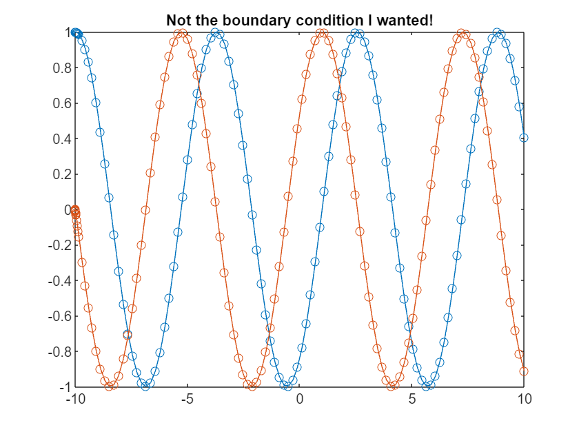
it applies the boundary condition and which is not the problem I wanted it to solve! Instead I have to make two calls to ode45 -- one that goes forwards in time and the other that goes backwards.
y0 = [1; 0]; % initial conditions: y1(0)=1, y2(0)=0
[tf,yf] = ode45(@(t,y)[y(2);-y(1)], [0 10],y0);
[tb,yb] = ode45(@(t,y)[y(2);-y(1)], [0 -10],y0);
plot([flipud(tb);tf],[flipud(yb);yf],"-o")
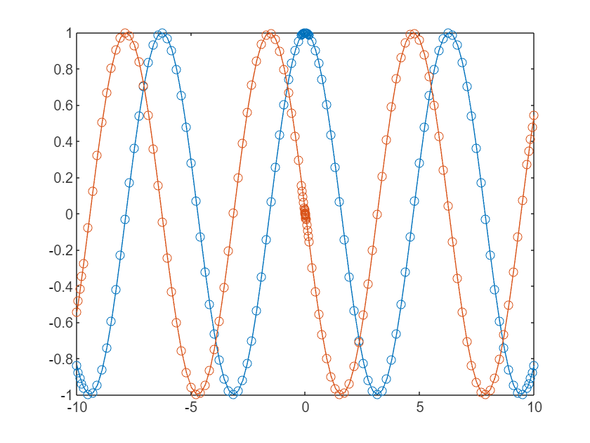
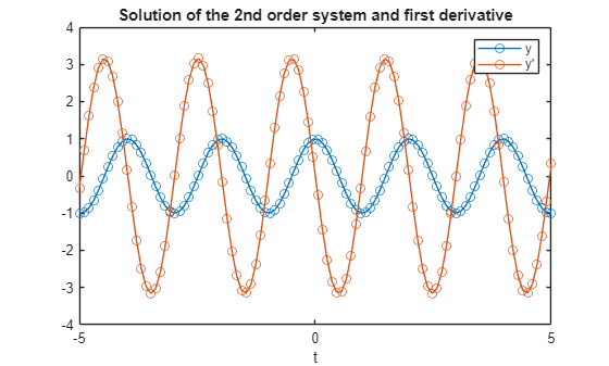
We got there but it took a couple of backflips. With the new interface, I don't need to worry about this as its much more flexible.
shm = ode(ODEFcn=@(t,y)[y(2);-y(1)],InitialTime=0,InitialValue=[1;0],Solver="ode45");
shmSol = solve(shm,-10,10);
plot(shmSol.Time,shmSol.Solution,'-o');
title("The same result but we got there more easily")
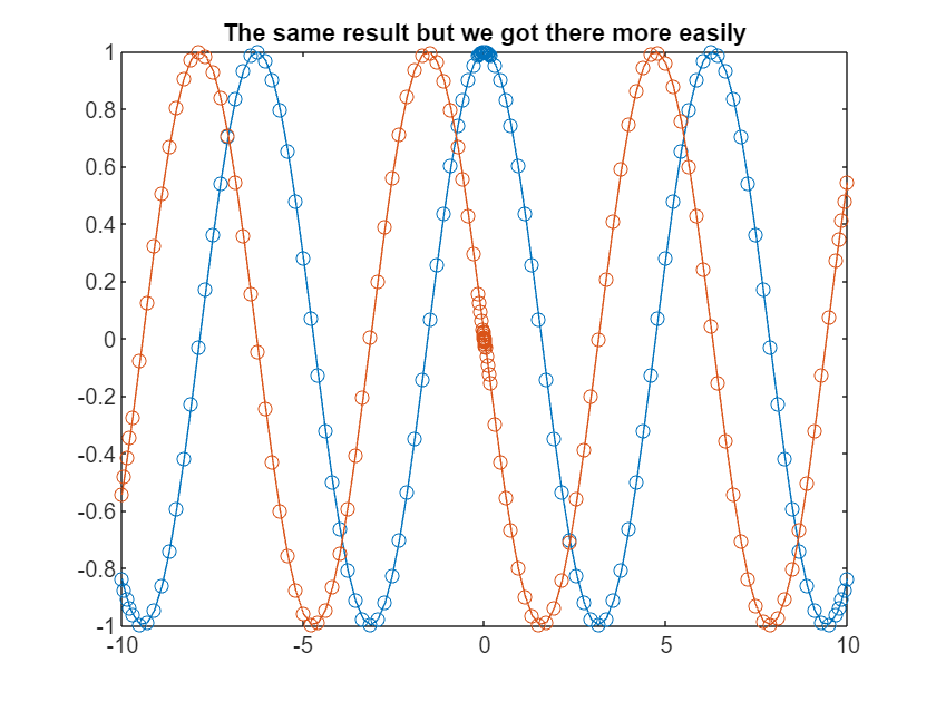
Unlike the traditional suite, the solution span we ask for doesn't even need to include our initial conditions.
% Request a solution span that doesn't include the initial conditions at t=0
shmSol2 = solve(shm,2*pi,4*pi)
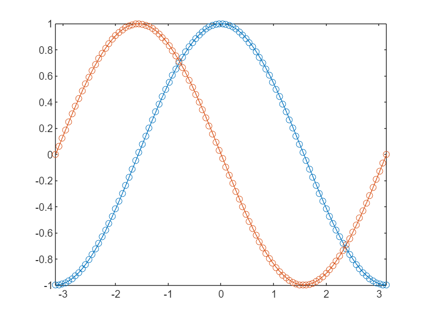
The closeness of the solution points around t = 0 is the solver starting the two integrations with a small initial step size. If we would rather choose the output points ourselves, we can just specify them.
shmSol3 = solve(shm,linspace(-pi,pi));
plot(shmSol3.Time,shmSol3.Solution,'-o');
xlim([-pi,pi]);
We can get all of these results using the traditional suite, of course, it's just that its easier and more intuitive now.
Event detection
Event detection has always been part of the MATLAB ODE suite and so, of course, this is also possible with the new framework. The documentation for ode demonstrates how to solve the classic bouncing ball problem using event detection. Here, I'll demonstrate how to use it to find maxima and minima of the solution to an ODE problem. The original problem comes from a 2011 blog post by John Kitchin.
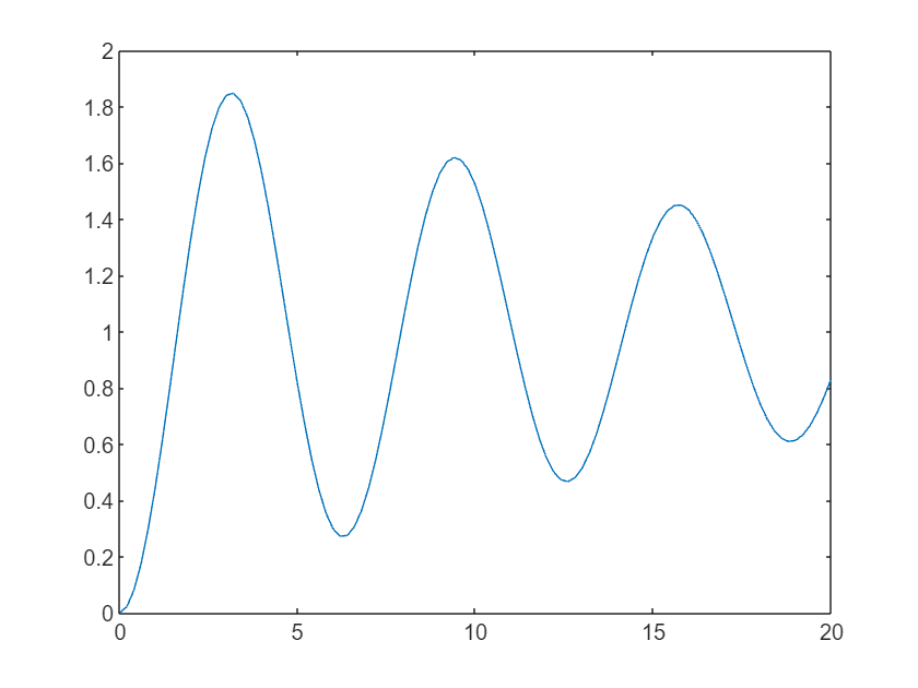
First, let's solve the ODE
myODE = ode(ODEFcn=@(t,y) exp(-0.05*t)*sin(t),InitialTime=0,InitialValue=0);
sol = solve(myODE,0,20,Refine=10);
plot(sol.Time,sol.Solution)
We want to find the maxima and minima of this solution. We know from calculus that these occur when our original equation is equal to zero.
odeEvent objects define events that the solver detects while solving an ordinary differential equation. An event occurs when one of the event functions you specify crosses zero.
So, we create an odeEvent object with an event function equal to our original ODE.
E = odeEvent(EventFcn = myODE.ODEFcn)
This time, let's solve the ODE with this event definition
myODE = ode(ODEFcn=@(t,y) exp(-0.05*t)*sin(t),InitialTime=0,InitialValue=0,EventDefinition=E);
sol = solve(myODE,0,20,Refine=10)
The solution includes all of the times the event occurs. Let's plot them
plot(sol.Time,sol.Solution,"-")
hold on
plot(sol.EventTime,sol.EventSolution,"ro")
hold off
xlabel("Time")
ylabel("y")
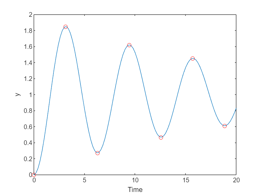
Exactly what we were looking for.
Obtaining the ODE solution as a function
Until now, we have been working with discrete representations of the solutions to our ODE problems and this can present limitations on further analysis. For example, what if we wanted to integrate the solution? What we need is a function that represents the solution and we can get one using solutionFcn, passing in the ode object we are aiming to solve.
myODE = ode(ODEFcn=@(t,y) exp(-0.05*t)*sin(t),InitialTime=0,InitialValue=0); % Define the ODE problem
solFcn = solutionFcn(myODE,0,20); % Use it to create a solutionFcn
I can now evaluate the solution at any point I like
solFcn(15)
or pass it to MATLAB's integral function
integral(solFcn,0,20)
Again, you could have done something similar with the old framework using deval and friends but I much prefer the new way!
Mass Matrices, Jacobians, Parameters and everything else I haven't covered here
This is just an introduction to the new framework and I encourage you to read the documentation to explore everything else it offers. Let me know what you think in the comments section.
- Category:
- MATLAB Programming Language,
- New Features,
- ode


See Also
-

A New View of Our Logo
Blogs


Comments
To leave a comment, please click here to sign in to your MathWorks Account or create a new one.