Creating natural textures with power-law noise: clouds, terrains, and more

Posted by Adam Danz, November 29, 2023

80 views (last 30 days) | 0 Likes | 8 comments

Today's guest writer is Adam Danz whose name you might recognize from the MATLAB Central community. Adam is a developer in the MATLAB Graphics and Charting team and the host of the Graphics and App Building blog. In this article he’ll share insights to creating structured noise and applying it to MATLAB graphics.

Noise is ubiquitous in nature. MATLAB has several tools to remove noise from data and images but in this article I'll review a method of generating noise that is currently being used by participants in the Flipbook Mini Hack contest to generate natural looking clouds, terrains, and textures including these examples below.

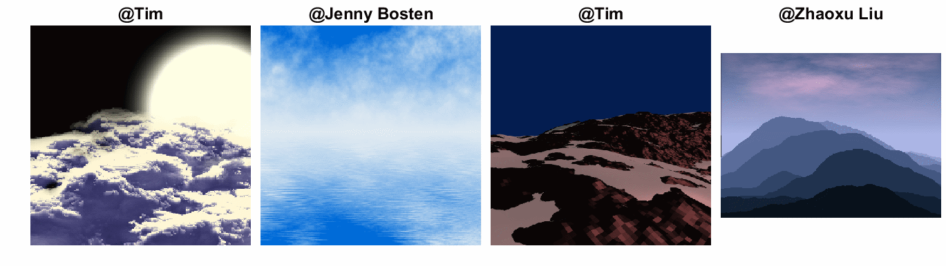
From left to right, Rolling fog, Blowin'in the wind, Morning ascent, landScape, from the 2023 MATLAB Flipbook Mini Hack contest.

This type of structured noise has several classifications including 1/f noise, coherent noise, fractal noise, colored noise, pink noise, fBm, and Brownian noise, each with their own definitions. For this article, I will refer to this type of noise as power-law noise, a term that describes the mathematical relationship between a signal's intensity and spatial or temporal frequency. Power-law noise can generate macro-scale variation such as hills and valleys while featuring micro-scale variation that adds texture. This type of noise is often found in natural phenomena from earthquakes to financial markets and it is quite easy to generate it in MATLAB.

Five Simple steps to generate 2D power-law noise in MATLAB

Creating power-law noise is surprisingly simple and requires only three parameters and a few lines of code in MATLAB. I'll walk you through the five steps depicted in the summary image below.

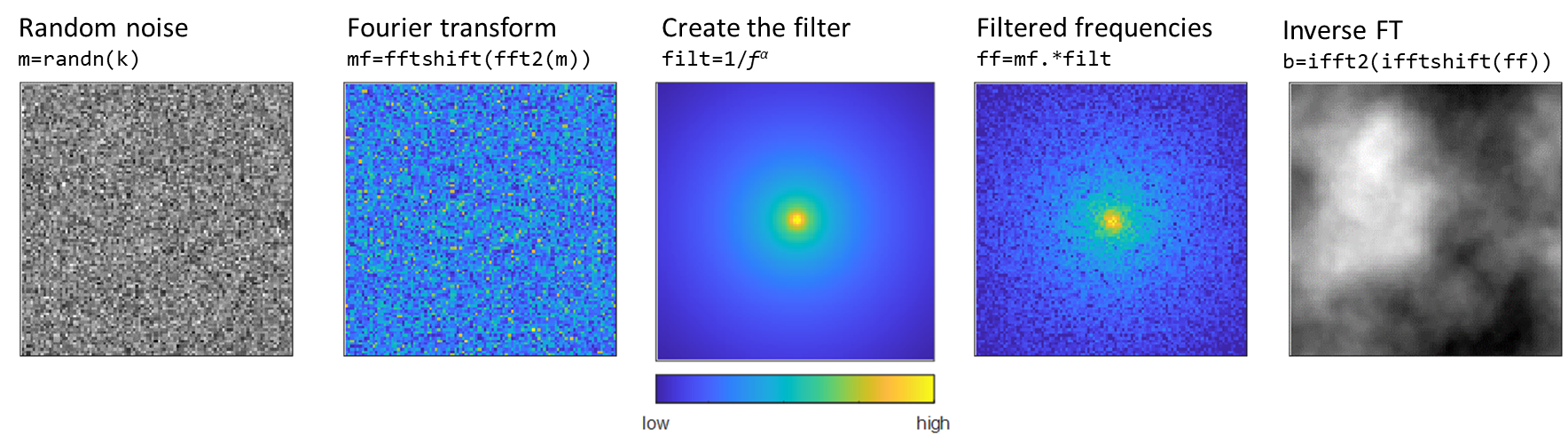
Summary of the five steps to creating 2D power-law noise

1. Random noise. Create a 2D matrix of random values. Some definitions of power-law noise require starting with Gaussian white noise which can be generated using randn() but uniformly distributed random numbers using rand() also produce fine results. The first two parameters are the size of the matrix and the random number generator seed (and generator type). Power-law noise is highly influenced by the initial values, so each seed and matrix size produces different results. The size parameter k must be even.

rng(0,'twister') % Parameter 1. random number generator seed

k = 100; % Parameter 2. size of the square matrix, must be an even scalar

m = randn(k); % k-by-k matrix

2. Fourier transform. Transform the 2D array from spatial to frequency domains using the 2D fast Fourier transform function fft2(). This returns a matrix of frequency coefficients in a pyramid arrangement where coefficients for low frequencies are on the perimeter of the matrix and coefficients for high frequencies are in the middle of the matrix. Step four requires an inversion of this arrangement where coefficients for low frequencies are in the middle and coefficients for high frequencies are on the perimeter of the matrix. Use fftshift() to invert the arrangement.

mf = fftshift(fft2(m));

How do I interpret the 2D frequency coefficients? This paragraph is for curious readers and for my personal challenge to concisely explain it. 2D Fourier transforms decompose an image into a set of planar sinusoidal waves at various frequencies and orientations. The frequency coefficients are complex numbers that provide a set of instructions for how to combine or superimpose the planar waves to recreate the image. Consider the value at mf(u,v). The real and imaginary components of mf(u,v) correspond to the amplitude and phase of the 2D sinusoidal plane that is defined by the frequencies assigned to row u and column v. Since MATLAB's image functions do not support complex values, the magnitudes of the frequency coefficients are shown in the second and fourth panels of the summary figure above. The magnitude of a complex numbers is computed using abs().

3. Create the filter. An important characteristic of power-law noise is the dominance of lower frequencies while still allowing higher frequencies to contribute to the variation. This creates macro patterns in the image such as 2D hills or cloud bellows while maintaining micro variations that add texture. In terms of frequency, sections of an image with fine details have high spatial frequency while smoother sections have low spatial frequency. The goal of the filter is to accentuate lower spatial frequencies in the image to create the macro patterns. Recall from step two that the shifted Fourier transform matrix mf is organized such that coefficients for lower frequency waves are in the center. The 2D filter, therefore, should have an inverse relationship to frequency ($ 1/f$ where $f = \sqrt{f_u^2 + f_v^2}$ for 2D signals) such that greater weight is placed on lower frequencies in the center and less weight on higher frequencies near the perimeter. The amount of emphasis placed on lower frequencies is controlled by the third parameter in this process, the exponent in $1/f^α$ which is typically within the range of 0<α<=3. Larger values of α result in greater influence from low spatial frequencies which result in smoother noise transitions with less detailed texture as shown in the image below. The value of α is used to define several classifications of noise such as white noise (α=0) pink noise (α=1) and Brownian noise (α=2).

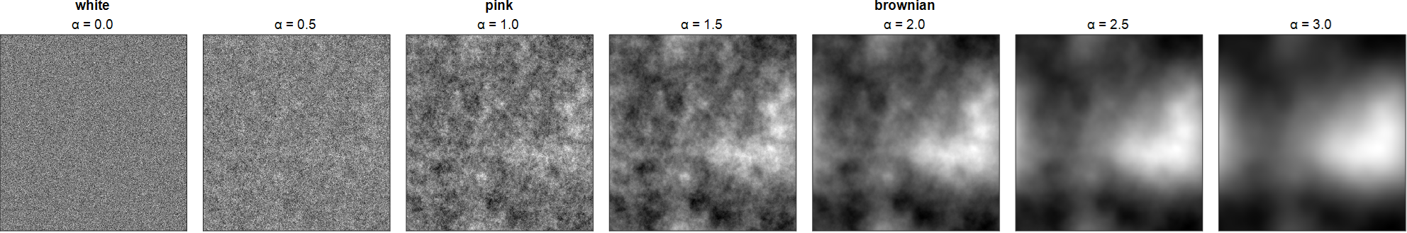
Exponent values are shown at the top of each image. Larger exponents result in smoother, lower frequency noise

Every implementation of power-law noise I've seen creates the filter differently but follows the same pattern of weight distribution. This filter is quite robust at returning real number values in step five, though it requires that k is even.

a = 2; % Parameter 3. 1/fᵅ exponent

d = ((1:k)-(k/2)-1).^2;

dd = sqrt(d(:) + d(:)');

filt = dd .^ -a; % frequency filter

filt(isinf(filt))=1; % replace +/-inf at DC or zero-frequency component

4. Filtered frequencies. Multiply the shifted Fourier transform matrix by the filter. Looking at the fourth panel of the 5-step summary image, it is difficult to imagine how this matrix contributes to the final image. We're used to thinking about matrices in the spatial domain where the value at coordinate (u,v) determines the intensity of the pixel at (u,v) of the image. Instead, this panel shows that lower spatial frequencies toward the middle of the matrix have higher coefficients which means that the lower spatial frequencies will have a greater effect on the final results.

ff = mf .* filt;

5. Inverse Fourier transform. We started with a matrix of random values. A Fourier transform reconstructed the random matrix in the frequency domain and the filter accentuated lower frequencies. The final step is to convert the filtered frequencies back to the spatial domain. Shift the frequencies back to their original pyramidal arrangement with coefficients for lower frequencies on the perimeter and coefficients for higher frequencies at the center using ifftshift(). Then apply a 2D inverse Fourier transform using iff2().

b = ifft2(ifftshift(ff));

The result (b) is a matrix of real numbers forming structured noise the same size as the original image. View the results shown in panel five of the 5-step summary image using imagesc(b) and apply a color bar to investigate the image's intensity values.

It is common to scale the noise values to a range of [-1,1] which makes it easier to apply additional customized scaling. To scale the results, use rescale().

bScaled = rescale(b,-1,1);

This pattern of applying a filter to a Fourier transformed image and then inversing the process back to an image is common in image processing and provides a nice model for learning about image filters.

Visualizing the power-law noise matrix.

The array of power-law noise values is commonly applied to color data, alpha value (transparency), or as height values in a 3D surface. The figure below shows the same noise matrix applied to four different visualizations.

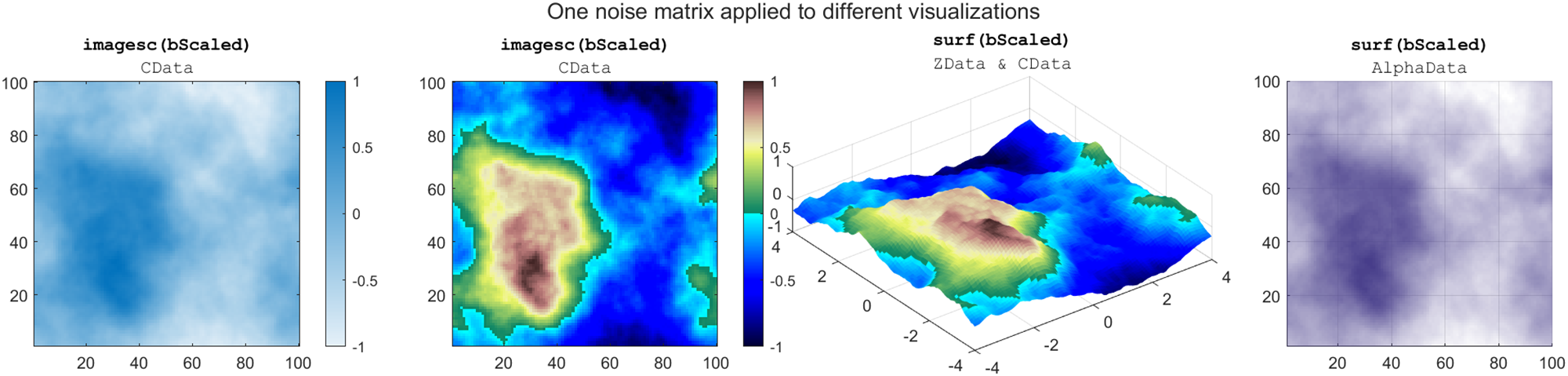
Applications of power-law noise in MATLAB graphics

To produces these panels, create the power-law noise matrix (bScaled) following the five steps above but replace the size parameter with k=500. Then continue with the code block below. The second and third panels use a custom colormap terrainmap which is attached to this article (download). Note that the Mapping Toolbox has an improved terrain colormap, demcmap.

% Panel 1

figure()

imagesc(bScaled)

set(gca,'YDir','normal')

colormap(gca,sky(256))

colorbar

%

% Panel 2

figure()

imagesc(bScaled)

set(gca,'YDir','normal')

colormap(gca,terrainmap()) % custom colormap

colorbar

%

% Panel 3

figure()

x = linspace(-4, 4, width(bScaled));

y = linspace(-4, 4, height(bScaled));

surf(x,y,bScaled,EdgeColor='none')

colormap(gca,terrainmap()) % custom colormap

axis equal

%

% Panel 4

figure()

s = surf(zeros(k,k),FaceColor=[.28 .24 .54],EdgeColor='none',...

    AlphaData=bScaled,FaceAlpha='flat');

view(2)

Use light to reveal texture

The texture provided by power-law noise can go unnoticed when there isn't sufficient color variation in the graphics object. The use of lighting in MATLAB reveals the texture by adding detailed shading to objects. The image below shows the same mountain as in the surface plot above. Water level was added as a planar surface with color defined by a second noise matrix. Light position was selected manually using the cameratoolbar tool and its values were extracted and placed in the code below for reproducibility. Camera properties were set to zoom in to the mountain.

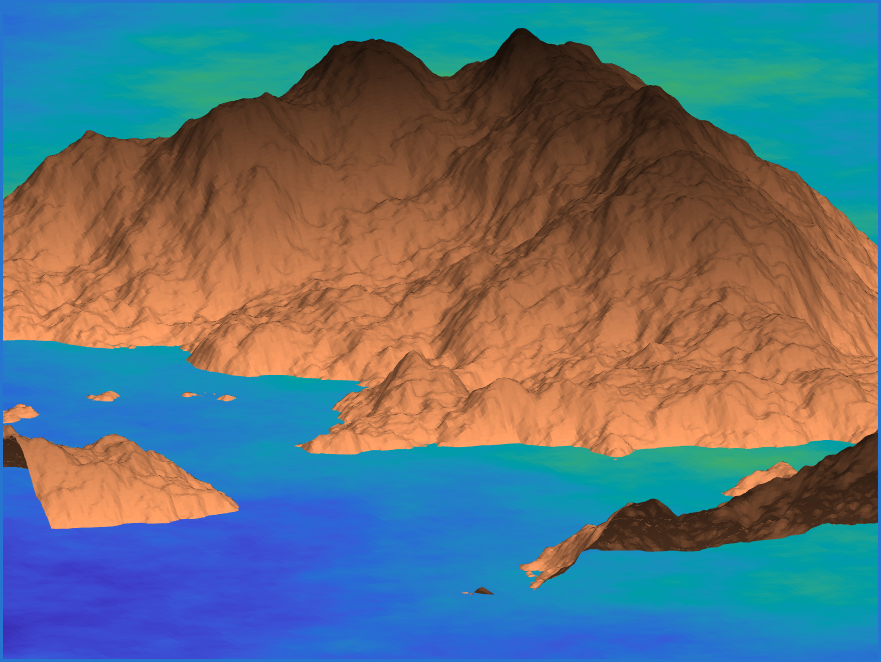
The use of lighting accentuates texture

rng(0,'twister')

k = 500;

mountainHeights = makenoise(k, 2); % mountain noise

figure()

x = linspace(-4, 4, k);

y = linspace(-4, 4, k);

mountainHeights = mountainHeights + 0.3; % raise the mountain

surf(x,y,mountainHeights,EdgeColor='none')

colormap(flipud(copper))

hold on

seaShading = makenoise(k, 1.5); % water color noise

nColors = 500; % number of colors to use for the water

seaColors = parula(nColors*3/2);

seaColors(nColors+1:end,:) = []; % Capture the blue-green end of parula

% convert seaShading (-1:1) to colormap indices (1:500)

seaShadingIdx = round((seaShading+1)*(nColors/2-.5)+1);

% Create mxnx3 matrix of CData

cdata = reshape(seaColors(seaShadingIdx,:),nColors,nColors,3);

S=surf(x*3, y*3, 0*seaShading,CData=cdata,EdgeColor='none');

axis equal off

clim([-0.5, 1.5])

light(Position = [-.8 .1 .75]) % add lighting

material dull

camva(10) % camera viewing angle

campos([-14 7 4]) % camera position

camtarget([.4 .8 .4]) % camera target

function noise = makenoise(k, a)

% Create the noise matrix

% k is the matrix size (scalar)

% a is the positive exponent (scalar)

% noise are noise values with range [-1,1]

m = randn(k);

mf = fftshift(fft2(m));

d = ((1:k)-(k/2)-1).^2;

dd = sqrt(d(:) + d(:)');

filt = dd .^ -a;

filt(isinf(filt))=1;

ff = mf .* filt;

b = ifft2(ifftshift(ff));

noise = rescale(b,-1,1);

end

Seamless tiling

Seamless tiling is another neat property of this style of noise. The edges of the matrix wrap seamlessly in a tiled arrangement as shown in the image below using the parula colormap.

figure()

tiledlayout(3, 3, TileSpacing='none', Padding='tight')

for i = 1:9

    nexttile()

    imagesc(bScaled)

    set(gca,'XTickLabel',[],'ytickLabel',[])

end

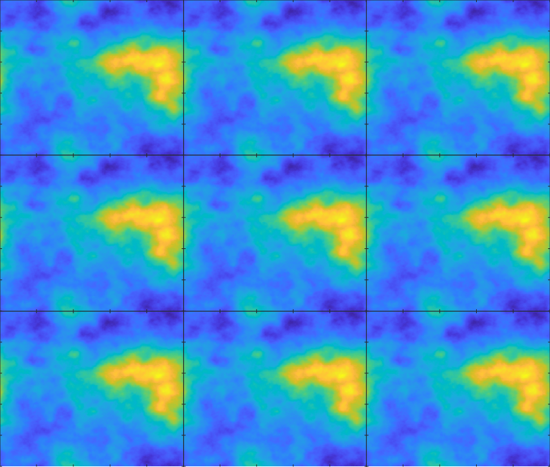
3x3 tile of the same noise matrix shows circular wrapping around its edges

Working in reverse: classifying noise by estimating the exponent

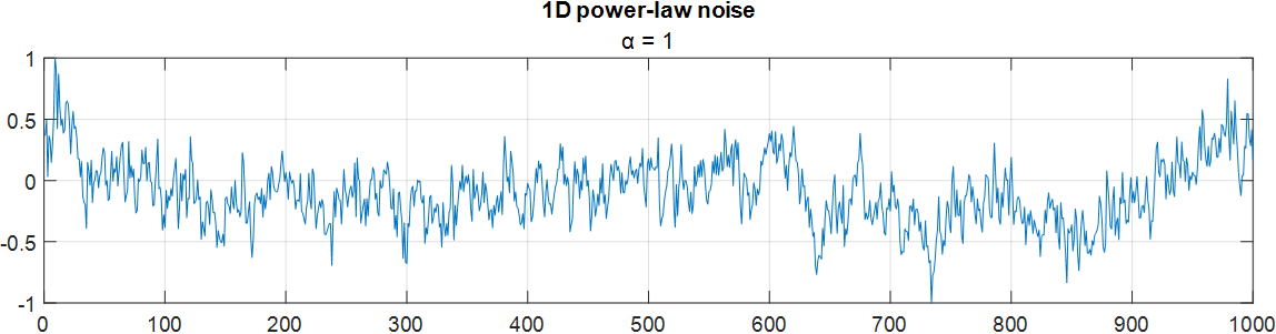
A 1D vector of power-law noise has the same macro-level hills and micro-level texture as the 2D case. This section below plots 1000 values of pink noise defined by an exponent of α=1.

rng default % Parameter 1. random number generator seed

k = 1000; % Parameter 2. size of the vector, must be even.

m = randn(k,1);

mf = fftshift(fft(m));

a = 1; % Parameter 3. 1/fᵅ exponent

d = sqrt(((1:k).'-(k/2)-1).^2);

filt = d .^ (-a/2); % frequency filter for 1D

filt(isinf(filt))=1;

ff = mf .* filt; % apply the filter

v = ifft(ifftshift(ff)); % power-law noise vector

vScaled = rescale(v,-1,1); % scaled power-law noise [-1,1]

figure()

plot(vScaled)

grid on

title('1D power-law noise')

subtitle('α = 1')

Suppose you start with the noise vector and you want to classify the color of the noise by its exponent value. The exponent can be approximated as the slope of the $1/f^α$ power spectrum in log-log coordinates. Fortunately, MATLAB's Signal Processing toolbox makes this task easy with the pspectrum function.

% Compute the power and frequency of the power-law noise vector

% Requires signal processing toolbox

[power, freq] = pspectrum(vScaled);

%

% Apply the log transform

freqLog = log(freq);

powerLog = log(power);

%

% Remove inf values

infrm = isinf(freqLog) | isinf(powerLog);

freqLog(infrm) = [];

powerLog(infrm) = [];

%

% Fit the relationship between log-power and log-frequency

% Requires the Curve Fitting toolbox

F = fit(freqLog,powerLog,'poly1');

%

% Plot the power density

figure()

plot(freqLog,powerLog)

%

% Add the linear fit

hold on

h = plot(F);

h.AffectAutoLimits = 'off';

grid on

axis tight

%

% Print the slope in the title

coeffs = coeffvalues(F);

xlabel('log frequency')

ylabel('log power spectrum')

title(sprintf('Slope = %.2f', coeffs(1)))

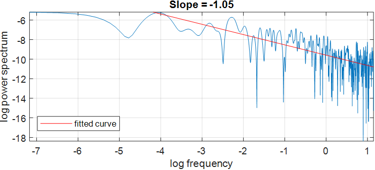
The slope of the linear fit is -1.05 which would correctly classify this signal as pink noise (α=1).

Summary points

Power-law noise such as pink and Brownian noise can be used to create 2D and 3D objects with naturally occurring noise variation.
Creating power-law noise matrices in MATLAB is quite simple and involves only five steps.
The basic principle of power-law noise creation involves filtering a Fourier transformed 2D matrix of random values by weighting the frequency coefficients by the inverse frequency and then applying an inverse Fourier transform.
A 2D power-law noise matrix can be applied to images and surfaces as color data, alpha data (transparency), height data, or as intensity values.
The use of lighting in MATLAB brings out the texture in surfaces.
Several MATLAB users have used this technique to create impressive images in the Flipbook Mini Hack contest which runs until December 3, 2023.

Additional resources

colored_noise is a wonderful tool on the File Exchange by Abhranil Das that creates power-law noise in any number of dimensions (also on git).
Abhranil Das' 2022 thesis on Camouflage Detection & Signal Discrimination (Ch. 5) contains a terrific interpretation of 2D Fourier transform coefficients.
Paul Bourke's 1998 articles on generating noise and applications in graphics is a source of inspiration and creativity.