Todays guest bloggers are Alex Silva da Purificação and Lucas Martins Ricardi from the University o f Brasília – Piratas do Cerrado Baja SAE Team. They will explain how they have utilized MATLAB for predicting the dynamic behavior of a continuously variable transmission (CVT).  

Introduction and Motivation 

The continuously variable transmission (CVT) is an automotive automatic transmission concept capable of varying the transmission ratio continuously, with the possibility of keeping the engine rotation constant, and thus its torque and power delivery. The use of CVT is quite common in Baja SAE teams, because of its ability to replace the use of the conventional clutch and the possibility of being adjusted for different applications.  

In this context, we from the Piratas do Cerrado Baja SAE team at the University of Brasília, have dedicated ourselves for several seasons in adjusting sets of flyweights and springs to define the best set up to provide better longitudinal performance for our car. However, over the years, this setup was carried out mostly on an experimental basis, which required a lot of testing time and financial resources. 

Therefore, in the last year, we decided to carry out an ambitious project as our graduation thesis, to develop an algorithm in MATLAB to predict the dynamic behavior of CVT, from the modeling of control mechanisms and belt. Consequently, it would be possible to change the inputs of mass and inertia of the flyweights, spring stiffness and analyze the outputs of secondary pulley rotation and torque. Thereby the CVT design and setup process become cheaper and less exhaustive.   

The original goal was to design our own CVT with this model, but after seeing the complexity and the various possibilities of the algorithm, we realized that to succeed we needed a full understanding of the model variables. Then, we scaled back to focus just on kinematic and dynamic analysis. 

We will try in the following topics to briefly present the methodology and results we obtained in the current phase of the development of our project, as well as future implementations and projects. 

Methodology 

In order to model the global CVT behavior, we divided the work into two different models, one for the belt and the other for the drive mechanism. For the first model, we discretized the belt in nodes joined by springs and dampers, then, the node position on the time is determined solving the force balance in each node. Figure 1 shows belt discretization and the forces considered acting on the nodes [1], and equation 1 the sum of forces in each node. 

Figure 1: Forces acting on the nodes [1] 

With the sum of forces in each node and dividing this by the mass, we have the dynamic equation of motion. Integrating equation 2 twice in time, we can find the position values of the nodes. 

Thus, with the input of primary pulley rotation data, axial force on the pulleys, and resistive torque submitted to the system, we are able to find the position and speed of each discretized nodes and consequently determine the rotation and torque on the secondary pulley. 

We use a mechanical CVT in our Baja, so the balance of forces between the springs and the centrifugal force under the flyweights generated by the rotation of the engine gives the Drive axial force, figure 2, which is input to the belt model. Thus, we developed a model for the control mechanism and coupled this system to the belt code.  

Figure 2: Free-body diagram on the primary pulley 

With that, we have all the models for the construction of our script. The flowchart in figure 3 shows the logic sequence of the algorithm. With the input of the initial conditions, we calculated the balance of forces, and with the Runge-Kutta method of solving differential equations, we have as output analysis the shift curves, torque on the secondary pulley, and belt position. 

Figure 3: Logical sequence of the algorithm 

In this way, we have a model capable of sensing the variation of the CVT control parameters, and thus we can analyze their interference in the results of coupling speed, output torque, and shift ratio. Consequently, the process of setting up our car is faster and less expensive, since we can test several combinations in MATLAB that would not be possible experimentally. 

Results and conclusion 

Running the complete model several analyzes can be performed. In video 1, it is possible to analyze the transmission behavior during the continuous variation of the shift ratio. As expected, the application of the axial force generated by the drive control mechanism induces a tight-side tension and a loose-side tension, which produces the transmission of torque to the secondary pulley.  

Video 1: Belt traction during continuous transmission variation 

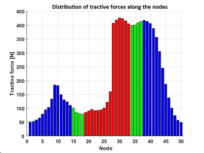
This difference in tension between the sides of the belt can be clearly seen in the distribution of tractive force along the nodes, figure 4. The regions in red are the nodes on the primary pulley, in blue the nodes on the secondary pulley, and in green the nodes outside the pulleys. 

Figure 4: Distribution of tractive force along the nodes – Nodes on the primary pulley (red), on the secondary pulley (blue), outside the pulleys (green). 

The slack dynamic behavior analysis during the transmission is very useful because it is possible to characterize the efficiency of the transmission, which is greatly influenced by the slip between the belt and the pulleys. This behavior would not be possible to analyze in a static model, without the discretization of the belt. 

The drive ratio curve in time, figure 5, is very important for us because this transmission variation determines the acceleration behavior of our car. This curve serves as input into a longitudinal dynamics algorithm that gives us the car’s speed and acceleration over time. 

Figure 5: Drive ratio over time 

With the implementation of this model in the dimensioning calculation of our project, it will be possible to simulate conditions that would not be possible experimentally. Furthermore, it provided us great evolutions in the theoretical knowledge about the dynamic behavior of the CVT, and how parameters such stiffness, mass, inertia, and pre-tension interfere in the longitudinal dynamics of the car. 

Future scope 

For the continuation of our work, we intend to implement this algorithm to the longitudinal dynamics model of the car already developed by the team. So, in the same program in MATLAB, will be possible to analyze the interference of the CVT adjustment parameters in the global acceleration behavior and speed of the entire vehicle. Besides, we hope in the future to carry out optimization analyzes of the control parameters based on fixed variables, to have the knowledge to develop our own CVT with design optimization for application in BAJA competitions. 

To get an update on our progress or take any questions about our dynamic CVT model, feel free to contact us on LinkedIn or the team’s Instagram. 

Thanks for reading and I hope you enjoyed it. Cheers! 

References 

[1] JULIO, G.; PLANTE, J.-S. An experimentally-validated model of rubber-belt cvt mechanics. Mechanism and Machine Theory – MECH MACH THEOR, v. 46, p. 1037–1053, 08 2011.