Spatial transformations: findbounds
I've written previously about how Image Processing Toolbox uses inverse mapping to implement spatial transforms. In this method, you set up a grid in output space. For each pixel in the output space grid, you use the inverse transform to determine the corresponding input space location, and you interpolate to get the input image pixel value at that point.
I've also written about the question of where to establish the grid in output space. If you don't somehow pay attention to the specific transformation, you might choose a grid that's too small:
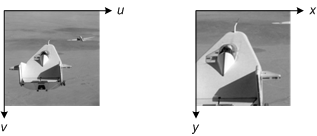
Or your grid might be too big:
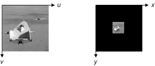
Or your grid might be in the wrong place completely:
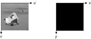
To avoid these problems (and to avoid the tech support calls!), the function imtransform uses the function findbounds to determine automatically where to place the output grid and how big it should be.
findbounds first creates a grid of points. These points are located in input space at each corner of the image, as well as in between each corner and in the middle. It looks like this:
I = imread('rice.png');
h = imshow(I);
set(h,'AlphaData',0.3);
axis on, grid on
in_points = [ ...
    0.5000    0.5000
    0.5000  256.5000
  256.5000    0.5000
  256.5000  256.5000
    0.5000  128.5000
  128.5000    0.5000
  128.5000  128.5000
  128.5000  256.5000
  256.5000  128.5000];
hold on
plot(in_points(:,1), in_points(:,2), '.', 'MarkerSize', 18)
hold off

findbounds then calls tformfwd to transform these points into output space. (For this example I'm going to construct an affine tform struct that combines scaling, rotation, shear, and a large translation.)
tform = maketform('affine', ...
    [1.1067 -0.2341 0; 0.5872 1.1769 0; 1000 -300 1]);
out_points = tformfwd(tform, in_points)
out_points =

  1.0e+003 *

    1.0008   -0.2995
    1.1512    0.0018
    1.2842   -0.3595
    1.4345   -0.0582
    1.0760   -0.1489
    1.1425   -0.3295
    1.2177   -0.1789
    1.2928   -0.0282
    1.3593   -0.2088
plot(out_points(:,1), out_points(:,2), '.', 'MarkerSize', 18)
axis ij, axis image
grid on
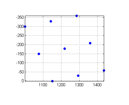
The bounding box of the points in output space tells us where to put the output space grid.
When you call imtransform, you can use optional output arguments to determine where the image is located in output space.
[J,XData,YData] = imtransform(I, tform);
XData
XData =

  1.0e+003 *

    1.0017    1.4337
YData
YData =

 -358.7527    1.2473
You can use this information together with imshow to place the image in the right place on an axes that contains other X-Y data.
h = imshow(J,'XData',XData,'YData',YData);
set(h,'AlphaData',0.3)
hold on
plot(out_points(:,1), out_points(:,2), '.', 'MarkerSize', 18)
axis on
grid on
hold off
axis ij, axis image

So that's the method imtransform uses to determine where the output image should be in output space.
In a future posting I'll cover two more topics related to findbounds and imtransform:
- What to do when there's no forward transform in the tform structure
- The special problem of pure translation
- カテゴリ:
- Spatial transforms




コメント
コメントを残すには、ここ をクリックして MathWorks アカウントにサインインするか新しい MathWorks アカウントを作成します。