Spatial transformations: Controlling the input and output grids with imtransform
The function imtransform has several optional parameters that allow you to fine-tune its behavior. Today's topic is about the parameters that let you control where the input image lives in input space, as well as the location and spacing of the output space pixel grid.
Contents
Input image location
imtransform assumes that an M-by-N input image lives in input space inside a rectangle spanning from 0.5 to M+0.5 horizontally, and from 0.5 to N+0.5 vertically.
I = checkerboard(1,4);
imshow(I, 'initialmag', 'fit')
axis on
box on
set(gca, 'XTick', [1 8], 'YTick', [1 8])
xlabel('u axis')
ylabel('v axis')
title('8-by-8 image')

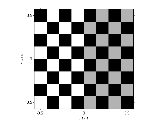
What if you want the input image to be in some other location? Sometimes, for example, it's convenient to place the center of the image at the input-space origin.
% imshow doesn't know about u-v space, just x-y space, so its parameters
% are called XData and YData.
imshow(I, 'XData', [-3.5 3.5], 'YData', [-3.5 3.5], 'initialmag', 'fit')
axis on
box on
set(gca, 'XTick', [-3.5 0 3.5], 'YTick', [-3.5 0 3.5])
xlabel('u axis')
ylabel('v axis')

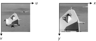
You can place imtransform's input image where you want in u-v space by specifying the UData and VData parameters. UData is a two-element vector. Its first value is the u-coordinate of the first column of the input image. Its second value is the u-coordinate of the last column. Similarly, VData is a two-element vector containing the v-coordinates of the first and last rows of the input image.
To place the center of an M-by-N image at the origin, specify UData to be [1 N] - (N+1)/2 and VData to be [1 M] - (M+1)/2.
Output space pixel grid
imtransform determines the bounding rectangle of the transformed image in output space and then overlays a pixel grid on that rectangle. The pixels in the output grid have the same size as the input image pixels.
You can modify the grid location and pixel size by specifying the XData, YData, and Size parameters in the call to imtransform.
XData and YData are similar to UData and VData. XData is a two-element vector containing the x-coordinates of the first and last columns of the output image. YData is a two-element vector containing the y-coordinates of the first and last rows of the output image.
The Size parameter is a two-element vector specifying how many rows and columns are in the output space grid.
Example
Here's your task: Position an input image centered at the origin and extending from -1 to 1 in the horizontal and vertical directions. Apply a 45 degree rotation to it. Compute the output image only inside a square extending from -0.8 to 0.8 horizontally and vertically. Also, compute the output image using only one-eighth as many pixels (in each direction) as the image input.
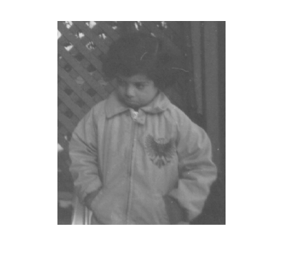
I = imread('pout.tif');
imshow(I)
T = [1 -sin(pi/4) 0; sin(pi/4) 1 0; 0 0 1];
tform = maketform('affine', T);

udata = [-1 1];
vdata = [-1 1];

xdata = [-0.8 0.8];
ydata = [-0.8 0.8];
output_size = round(size(I)/8);

J = imtransform(I, tform, 'UData', udata, 'VData', vdata, ...
    'XData', xdata, 'YData', ydata, 'Size', output_size);

imshow(J)

In an upcoming post I'm going to demonstrate how to define and apply custom spatial transformations. This post will include more examples illustrating the use of UData, VData, XData, and YData.


댓글
댓글을 남기려면 링크 를 클릭하여 MathWorks 계정에 로그인하거나 계정을 새로 만드십시오.