Dilation, erosion, and the morphological gradient
The morphological operator dilation acts like a local maximum operator. Erosion acts like a local minimum operator. You can use them together to compute something called the morphological gradient.
Contents
Dilation
The basic form of grayscale image dilation computes, for each image pixel, the maximum value of its neighboring pixels. The neighborhood is defined by the structuring element. For example, this structuring element:
se1 = strel([1 1 1])
se1 =

Flat STREL object containing 3 neighbors.

Neighborhood:
     1     1     1
defines a neighborhood consisting of the pixel itself, together with its left and right neighbors. Whereas this structuring element:
se2 = strel([1; 1; 1])
se2 =

Flat STREL object containing 3 neighbors.

Neighborhood:
     1
     1
     1
defines a neighborhood consisting of the pixel itself, together with the pixels above and below it.
Let's try dilation on everyone's favorite sample MATLAB matrix, the magic square:
m5 = magic(5)
m5 =

    17    24     1     8    15
    23     5     7    14    16
     4     6    13    20    22
    10    12    19    21     3
    11    18    25     2     9
d1 = imdilate(m5, se1)
d1 =

    24    24    24    15    15
    23    23    14    16    16
     6    13    20    22    22
    12    19    21    21    21
    18    25    25    25     9
d1(3,3), which is 20, is the maximum of [m5(3,2), m5(3,3), m5(3,4)], or [6 13 20].
Dilating with se2 computes the 3-pixel local maximum vertically:
d2 = imdilate(m5, se2)
d2 =

    23    24     7    14    16
    23    24    13    20    22
    23    12    19    21    22
    11    18    25    21    22
    11    18    25    21     9
d2(3,3) is the maximum of [m5(2,3), m5(3,3), m5(4,3)].
Erosion
Grayscale image erosion computes the minimum of each pixel's neighborhood.
e1 = imerode(m5, se1)
e1 =

    17     1     1     1     8
     5     5     5     7    14
     4     4     6    13    20
    10    10    12     3     3
    11    11     2     2     2
e1(3,3) is the minimum of [m5(3,2), m5(3,3), m5(3,4)].
Morphological gradient
Dilation and erosion are often used in combination to produce a desired image processing effect. One simple combination is the morphological gradient. P. Soille, in section 3.8 of the second edition of Morphological Image Analysis: Principles and Applications, talks about three kinds of basic morphological gradients:
- dilated_image - eroded_image
- original_image - eroded_image
- dilated_image - original_image
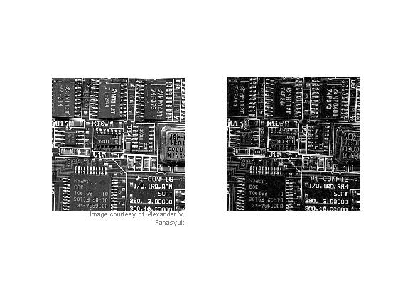
Soille calls the first one the basic morphological gradient, and you compute it this way using MATLAB and the Image Processing Toolbox:
% Read in circuit board image, crop it so it's not too big for the blog
% page, and convert it to grayscale:

rgb = imread('board.tif');
I = rgb2gray(rgb(1:256,1:256,:));

se = strel(ones(3,3));
basic_gradient = imdilate(I, se) - imerode(I, se);

subplot(1,2,1), imshow(I), imcredit('Image courtesy of Alexander V. Panasyuk')

subplot(1,2,2), imshow(basic_gradient, [])

The second form is called the half-gradient by erosion or internal gradient.
internal_gradient = I - imerode(I, se);

subplot(1,2,2), imshow(internal_gradient, [])

"The internal gradient enhances internal boundaries of objects brighter than their background and external boundaries of objects darker than their background. For binary images, the internal gradient generates a mask of the internal boundaries of the foreground image objects." [Soille, page 86]
The third form is called the half-gradient by dilation or external gradient:
external_gradient = imdilate(I, se) - I;
Direction gradients
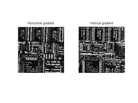
By using line segments as structuring elements, you can compute directional gradients.
seh = strel([1 1 1]);
sev = strel([1;1;1]);

horizontal_gradient = imdilate(I,seh) - imerode(I,seh);
vertical_gradient = imdilate(I,sev) - imerode(I,sev);

subplot(1,2,1)
imshow(horizontal_gradient, []), title('Horizontal gradient')

subplot(1,2,2)
imshow(vertical_gradient, []), title('Vertical gradient')

Try this on your own grayscale images. You can experiment with larger structuring elements, too, such as strel('disk',7).
I'll be covering ways to combine erosion, dilation, and other fundamental morphological operators in the near future.


评论
要发表评论,请点击 此处 登录到您的 MathWorks 帐户或创建一个新帐户。