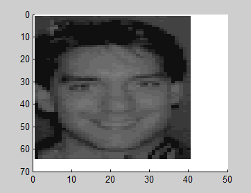
When MATLAB 5 was released, some users noticed that the default image had changed.

image
colormap(gray(32))
axis ij

A few users also noticed that the pixel values in the new default image were not integers.

h = findobj(gcf,'type','image');
cdata = get(h,'CData');
cdata(1:3,1:3)

ans =

   11.2307   12.4251   10.4251
   14.4251   15.7483   13.7483
   12.3938   13.7483   12.7483

Is there something interesting about the fractional part?

imagesc(cdata - floor(cdata))

Apparently so.

I now confess - you can blame me for all of this. I told this story in public for the first time last week at the IEEE International Conference on Image Processing in Atlanta, GA. Now, dear blog readers, you get to hear it, too.

I joined The MathWorks toward the end of 1993. Sometime in 1994, the company held its first employee charity auction. One of the "items" put up for bid was the right to choose the default image for MATLAB 5, which was then under development. As the new "image processing guy" in development, I felt some responsibility to bid. (At least, that's the way I tried to explain it later to my wife.) As it turned out, another MathWorks developer really wanted to win this item, so to win it I ended up paying big bucks. (It's all for charity, I kept reminding myself.)

Once I won the auction, I had to decide what image to pick. During this time, I frequently heard complaints from users that MATLAB could only handle double-precision values. (That lasted until 1997.) Because I heard so much about this issue, I decided that I would use all of the mantissa bits for the new default image. I solicited ideas from my fellow developers for what to include.

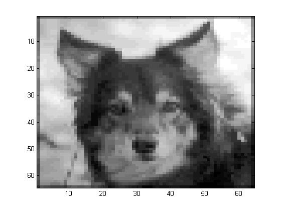
Here are the various images "hidden" in different bit slices of the default image pixel values. (To run the code yourself, download this little utility function, bitslice.)

The image stored in the 5 most-significant bits is the one you usually see. This is my oldest son.

defimage = pow2(get(0,'DefaultImageCData'),47);
mag = 200;
imshow(bitslice(defimage,47,51));

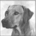
The next 5 bits show a dog that belonged to a MathWorks developer.

imshow(bitslice(defimage,42,46));

Here's another MathWorks pet.

imshow(bitslice(defimage,37,41));

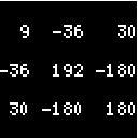
This famous matrix is the inverse of the 3-by-3 Hilbert matrix.

imshow(bitslice(defimage,36,36));

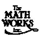
This is a low-resolution version of the company's original logo.

imshow(bitslice(defimage,35,35));

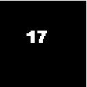
Loren's favorite number.

imshow(bitslice(defimage,34,34));

3-by-3 magic square.

imshow(bitslice(defimage,33,33));

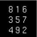
My youngest son.

imshow(bitslice(defimage,28,32));

A famous magic square hidden in Albrecht Durer's Melancolia.

imshow(bitslice(defimage,23,27));

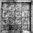
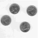
I couldn't resist a kind of visual pun. This is the original MATLAB "eight-bit image." (That'll tell you something about my sense of humor.)

imshow(bitslice(defimage,18,22));

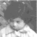
Loren at age 4.

imshow(bitslice(defimage,13,16));

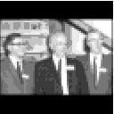
Wilkinson, Givens, and Forsythe, from the 1964 Gatlinburg Conference on Numerical Algebra.

imshow(bitslice(defimage,9,12));

Me.

imshow(bitslice(defimage,5,8));

The original default image from MATLAB 4 is still in there.

imshow(bitslice(defimage,1,4));

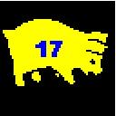
Finally, a certain combination of three bit slices makes a yellow pig with the number 17 superimposed on it. I've been told this is some sort of secret joke within a certain mathematical community.

r = bitslice(defimage,0,0);
g = bitslice(defimage,17,17);
b = bitslice(defimage,34,34);
imshow(cat(3,r,g,b));

There you have it - the complete story of the MATLAB default image.

function b = bitslice(a,lowbit,highbit)
% BITSLICE(A,LOWBIT,HIGHBIT)
%
%   Scales return values so that the maximum is 1.0.

b = a / 2^(lowbit);
b = fix(b);
b = b / 2^(highbit - lowbit + 1);
b = b - fix(b);

b = b / max(b(:));
end

Published with MATLAB® R2021a