Filling holes in images
Didja know? You can fill holes, or pits, in grayscale images by using the Image Processing Toolbox function imfill.
The other day I was rereading the Tarboton paper on upslope area, trying to decide what to do next in my series on that topic. I noticed that the author described filling in "pits" in digital elevation models (DEMs) as a common preprocessing step. He outlined a method based on pixel flow directions, but didn't give details. I realized that this preprocessing step is very easy to do using the Image Processing Toolbox, but that many users might not know about this capability.
Let me first define a little more precisely what I mean by "pit" or "hole," and then I'll show you how to fill it in. It's a little easier to show in one dimension, so let's start there.
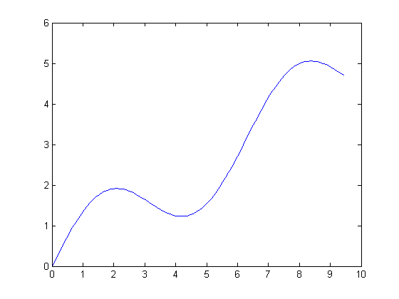
Here's a one-dimensional function:
t = linspace(0, 3*pi, 100);
y = t/2 + sin(t);
plot(t,y)

The plot above has a local minimum in its interior. This is a hole, or pit. If we are careful to define our connectivity appropriately for one dimension, we can use imfill with the 'holes' option to fill in the hole.
% Define a one-dimensional connectivity in the horizontal direction.
conn = [0 0 0; 1 1 1; 0 0 0];
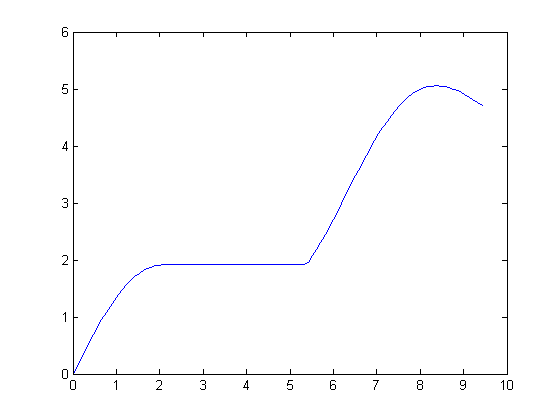
y2 = imfill(y, conn, 'holes');

plot(t,y2)

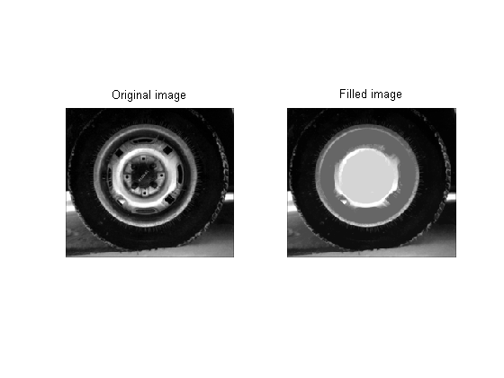
The filled curve has this key property: From any interior point, you can now travel to a boundary minimum without ever going uphill. Here's what it looks for an image:
I = imread('tire.tif');
I2 = imfill(I,'holes');  % the default connectivity is fine
subplot(1,2,1)
imshow(I)
title('Original image')
subplot(1,2,2)
imshow(I2)
title('Filled image')

The hole-filling algorithm in imfill is based on morphological reconstruction (imreconstruct). If you are interested in the theoretical details, see section 6.3.7 of Morphological Image Analysis: Principles and Applications, 2nd ed., Springer, by P. Soille.


댓글
댓글을 남기려면 링크 를 클릭하여 MathWorks 계정에 로그인하거나 계정을 새로 만드십시오.