Image overlay using transparency
Last August I posted an example showing how to display patch objects transparently over an image. I meant to follow that up with another post showing a couple of ways to display one image transparently over another. I was embarrassed to discover recently that I had completely forgotten to post the follow-up.
So here it is!
Handle Graphics image objects can be displayed transparently. In fact, each individual pixel can be assigned a different level of transparency. This can be used in various ways to view one image on top of another. In my first example for today, I'll use a "checkerboard" transparency pattern to view a gray-scale image on top of the original color image.
First, display the color image and the gray-scale image together, in the same place.
rgb = imread('peppers.png');
imshow(rgb);
I = rgb2gray(rgb);
hold on
h = imshow(I); % Save the handle; we'll need it later
hold off
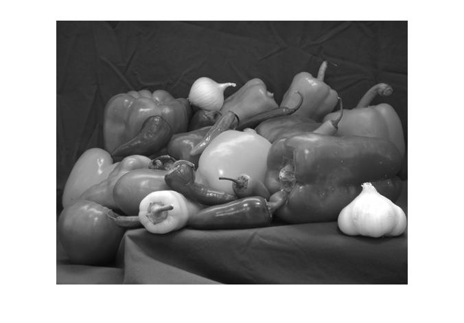
Not too surprisingly, only the gray-scale is visible. That's because it's "covering up" the color image. Let's give it a "checkerboard" transparency pattern, so that some of the pixels are fully opaque, and others are fully transparent.
[M,N] = size(I);
block_size = 50;
P = ceil(M / block_size);
Q = ceil(N / block_size);
alpha_data = checkerboard(block_size, P, Q) > 0;
alpha_data = alpha_data(1:M, 1:N);
set(h, 'AlphaData', alpha_data);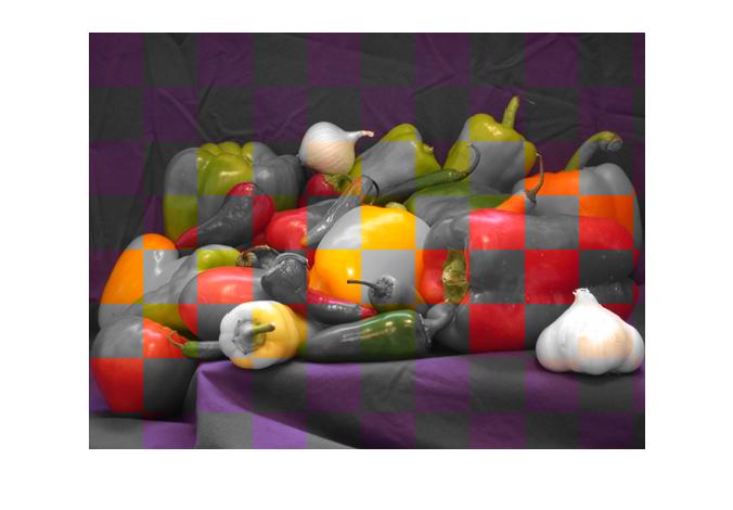
Now we can see some of both images. This visualization technique is often used to evaluate image fusion algorithms.
Using image data to control transparency
My second transparency example gets a bit more creative. I'll display an image that's a solid color, but I'll use another data set to vary the solid color image's transparency on a pixel-by-pixel basis.
Here's a digital elevation model (DEM) of Peppercorn Hill and North Pond in Massachusetts.
E = imread('peppercorn_hill.png');
imshow(E, 'InitialMag', 'fit')
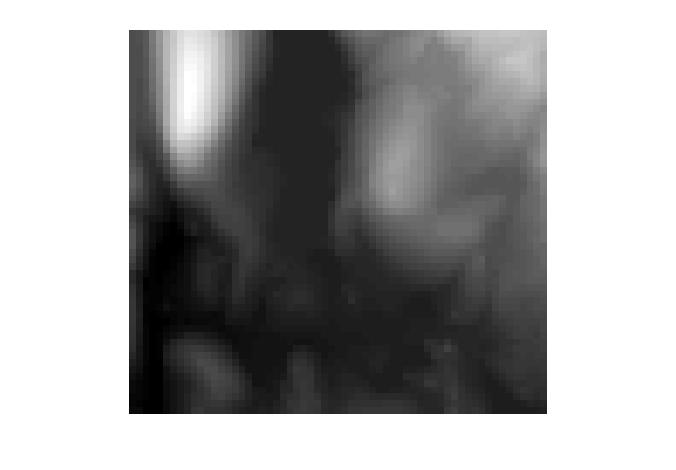
The bright blob at the upper left is Peppercorn Hill, and the flat, dark plateau in the upper middle is North Pond.
Below is an "influence map." This is a visualization of down-hill water flow, starting from the peak of Peppercorn Hill.
I = imread('peppercorn_hill_influence_map.png');
imshow(I, 'InitialMag', 'fit')
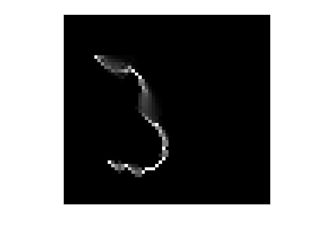
It's difficult to interpret the influence map image on its own, apart from the original DEM. Let's visualize the two images together as follows:
- Display the original DEM image.
- Display a solid green "image" on top of the original image.
- Use the influence map pixels to control the transparency of each pixel of the green image.
imshow(E, 'InitialMag', 'fit')

% Make a truecolor all-green image.
green = cat(3, zeros(size(E)), ones(size(E)), zeros(size(E)));
hold on
h = imshow(green);
hold off

% Use our influence map image as the AlphaData for the solid
% green image.
set(h, 'AlphaData', I)
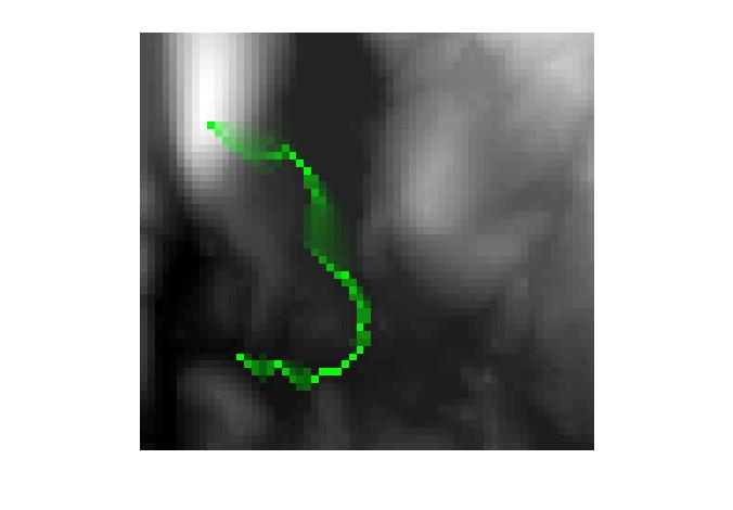
Now it's easy to understand the water flow in the context of the original DEM image. We can see that the water flows from the peak into the pond, then out the southern end of the pond.
So there you go, better late than never. Two more image visualization techniques to add to your bag of tricks.




评论
要发表评论,请点击 此处 登录到您的 MathWorks 帐户或创建一个新帐户。