MATLAB image display – scaled indexed images
In my last post on pixel colors, I described the truecolor and indexed image display models in MATLAB, and I promised to talk to soon about a third model. That model is the scaled indexed image, a variation on the indexed image. The function imagesc is often used to display a scaled indexed image.
Let me start by displaying a small magic square using the image function, and then I'll compare with a display using imagesc.
A = magic(5)
A =

    17    24     1     8    15
    23     5     7    14    16
     4     6    13    20    22
    10    12    19    21     3
    11    18    25     2     9
Let's display A using image and a 256-color grayscale colormap.
image(A)
colormap(gray(256))
axis image
axis ij
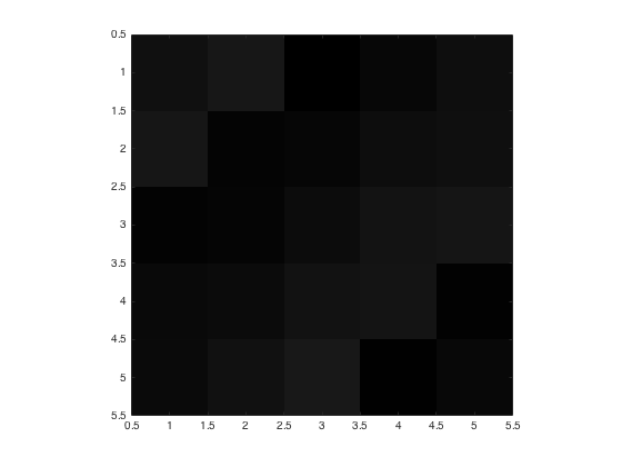
Notice the displayed image is very dark. That's because the values of A vary between 1 and 25, and so the image uses only the first 25 colors of the grayscale colormap, all of which are very dark.
Now compare with the display using imagesc:
imagesc(A)
colormap(gray(256))
axis image
axis ij
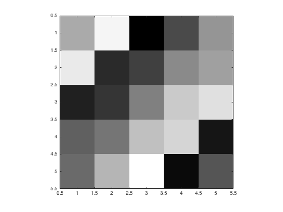
The function imagesc displays the lowest value of A, which is 1, using the first colormap color, which is black. It displays the highest value A, which is 25, using the last colormap color, which is white. All the other values between 1 and 25 are mapped linearly onto the colormap. For example, the value 12 is displayed using the 118th colormap color, which is an intermediate shade of gray.
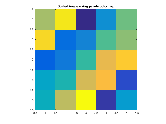
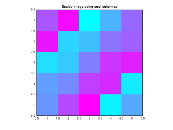
If you switch colormaps, the values of A will be scaled and displayed using the colors in the new colormap.
colormap(parula)
title('Scaled image using parula colormap')
colormap(cool)
title('Scaled image using cool colormap')
Now let's look at the graphics object properties that control this behavior. The functions image and imagesc both return an Image object if you call them with an output argument. (I'll close the figure so it isn't displayed here. For the moment, I just want to look at the Image object that gets returned.)
im1 = image(A)
close
im1 =

  Image with properties:

           CData: [5x5 double]
    CDataMapping: 'direct'

  Use GET to show all properties
Image objects have a property called CDataMapping. The image function creates an Image object with the CDataMapping property set to 'direct' by default. With this setting, values of A are used directly as indices into the colormap.
Compare that with the Image object created using imagesc.
im2 = imagesc(A)
close
im2 =

  Image with properties:

           CData: [5x5 double]
    CDataMapping: 'scaled'

  Use GET to show all properties
The imagesc function creates an image whose CDataMapping property is 'scaled'. Values of A are scaled to form indices into the colormap. The specific formula is:
$$k = \lfloor m (A_{ij} - c_{\min} / (c_{\max} - c_{\min}) \rfloor + 1$$
$A_{ij}$ is a value of an element of A, and $c_{\min}$ and $c_{\max}$ are the color limits. These limits come from the 'CLim' property of the Axes object. Here's how to view the color limits.
h = imagesc(A);
ax = gca;
ax.CLim
close
ans =

     1    25
It's not a coincidence that the the CLim property contains the minimum and maximum values of A. The imagesc function does that by default. But you can also specify your own color limits using an optional second argument to imagesc.
imagesc(A,[10 15])
colormap(gray)
title('imagesc(A,[10 15])')
axis image
axis ij
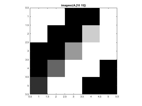
In the image above, the value 10 (and also lower values) were displayed as black. The value 15 (and also greater values) were displayed as white. Values between 10 and 15 were displayed as shades of gray.
Scaled image display is very important for engineering and scientific applications of image processing because we are often looking at something that is not a "picture" in the ordinary sense. Rather, it's often an array containing measurements in some physical unit that's not related to light intensity. For example, I showed this image in my first image display post earlier this month:
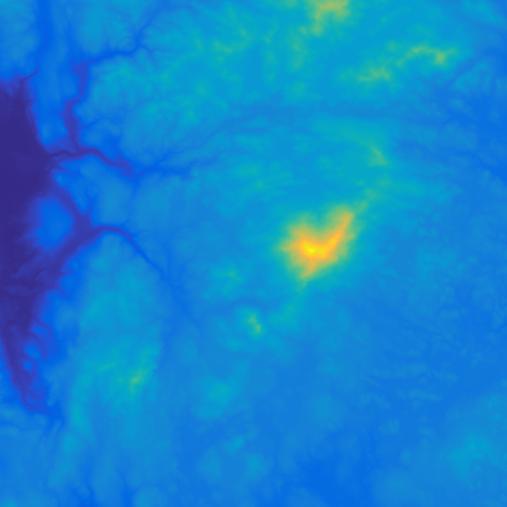
This is a scaled-image display of a matrix containing terrain elevations in meters.
Next time I'll talk about grayscale and binary images.
- Category:
- Pixel colors




Comments
To leave a comment, please click here to sign in to your MathWorks Account or create a new one.