Upslope area – Flow examples
In Part 2 of the upslope area series, I showed an M-file, pixelFlow, that could calculate a pixel's flow direction and magnitude according to the D-infinity method of Tarboton.
Let's try the function with a simple test case first, and then we'll try it with some DEM data.
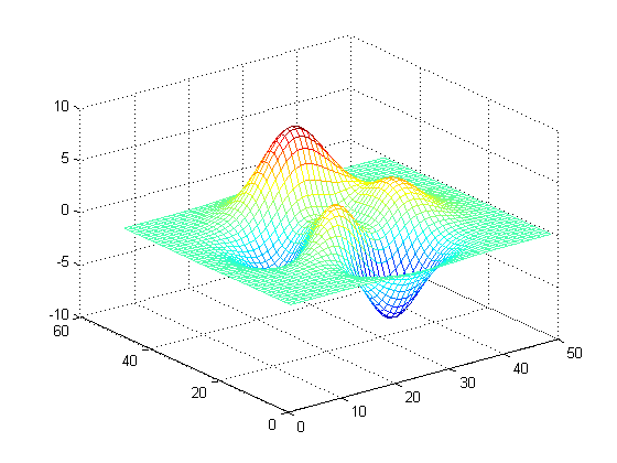
Z = peaks;
mesh(peaks)

pixelFlow works on a single pixel at a time, so we put it into a loop to calculate the flow direction, r, and the flow magnitude, s, for all the interior elements of Z.
[M,N] = size(Z);
r = zeros(M-2, N-2);
s = zeros(M-2, N-2);
for i = 1:M-2
    for j = 1:N-2
        [r(i,j), s(i,j)] = pixelFlow(Z,i+1,j+1);
    end
end
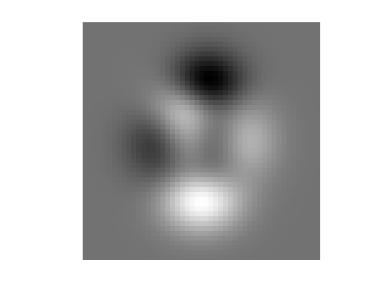
Now display the peaks matrix as a grayscale image and superimpose a quiver plot.
imshow(peaks,[],'initialmag','fit')
hold on
[x,y] = meshgrid(2:N-1,2:M-1);
quiver(x, y, s.*cos(r), -s.*sin(r), 2, 'y')
axis equal
hold off

Zoom in on a low point:
xlim([20 35]);
ylim([5 20])

And a high point:
xlim([30 40])
ylim([15 30])

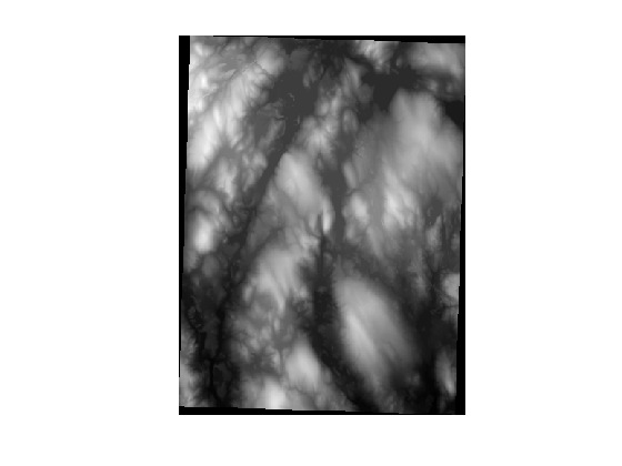
To get a real digital elevation model (DEM) to play with, I started at a page that the Mapping Toolbox development team fondly calls Tech Support Note 2101: "Accessing Geospatial Data on the Internet for the Mapping Toolbox." That page directed me to GeoCommunity, one of the distribution points for free DEM data from the United States Geological Survey (USGS). Downloading DEM data set 1643091 and using the Mapping Toolbox function sdtsdemread gave me this data set:
s = load('upslope_sample_dem');
imshow(s.Zm, [], 'initialmag', 'fit')

Near the center of this data set is North Pond, close to where I live and about 3 miles southwest of the Boston Marathon starting line. (The high spot west of the pond is Peppercorn Hill, a great place for a Cub Scout hike.)
pond = s.Zm(140:280, 160:230);
imshow(pond, [], 'initialmag', 'fit')
title('North Pond')

Let's try pixelFlow on this data set.
[M,N] = size(pond);
r = zeros(M-2, N-2);
s = zeros(M-2, N-2);
for i = 1:M-2
    for j = 1:N-2
        [r(i,j), s(i,j)] = pixelFlow(pond,i+1,j+1);
    end
end

imshow(pond,[],'initialmag','fit')
hold on
[x,y] = meshgrid(2:N-1,2:M-1);
quiver(x, y, s.*cos(r), -s.*sin(r), 2, 'y')
axis equal

% Zoom in on the southern end of the pond.
xlim([15 60])
ylim([75 105])

hold off

That seems to be working pretty well, but there's an unresolved problem to explore - what to do about plateaus. Recall the last few lines of pixelFlow:
dbtype pixelFlow 47:51
47    else
48        % The pixel is in a flat area or is a pit.  Flow direction angle is
49        % unresolved.
50        r = NaN;
51    end
For example:
Zp = repmat([1:3 3 3 3:6],5,1)
Zp =

     1     2     3     3     3     3     4     5     6
     1     2     3     3     3     3     4     5     6
     1     2     3     3     3     3     4     5     6
     1     2     3     3     3     3     4     5     6
     1     2     3     3     3     3     4     5     6
r = zeros(size(Zp)-2);
for i = 1:size(r,1)
    for j = 1:size(r,2)
        r(i,j) = pixelFlow(Zp, i+1, j+1);
    end
end

r
r =

    3.1416    3.1416       NaN       NaN       NaN    3.1416    3.1416
    3.1416    3.1416       NaN       NaN       NaN    3.1416    3.1416
    3.1416    3.1416       NaN       NaN       NaN    3.1416    3.1416
The pixel flow direction is to the left (r = pi) except for the middle pixels, for which pixelFlow could not compute a direction.
I'll pursue the issue of plateaus next week.
- Category:
- Upslope area


Comments
To leave a comment, please click here to sign in to your MathWorks Account or create a new one.