Binary image convex hull – algorithm notes
Today I want to tell a little image processing algorithm story related to my post last week about the new bwconvhull function in the Image Processing Toolbox.
The developer (Brendan) who worked on this function came to see me sometime last year to find out how the 'ConvexImage' measurement offered by regionprops was computed so that he could use the same procedure for bwconvhull. I believed that I knew the answer off the top of my head, so without looking at the code I rattled off the following steps:
A few days later Brendan came back to tell me that, although my description was clear, the code that I wrote ten years ago for regionprops actually does something else.
Oops.
I looked at the code and realized that Brendan was right, and I started to remember that I had actually made this same mistake many years before.
In fact, I did originally implement 'ConvexImage' in regionprops using the procedure outlined above. Before it shipped, though, I discovered (and fixed) a big problem with it.
Let me show you the problem using a small example. Here's a tiny binary image.
bw = [...
    0 0 0 0 0 0 0 0 0
    0 0 0 0 1 0 0 0 0
    0 0 0 1 0 1 0 0 0
    0 0 1 0 0 0 1 0 0
    0 1 0 0 0 0 0 1 0
    0 0 0 0 0 0 0 0 0 ];
imshow(bw, 'InitialMagnification', 'fit')

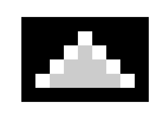
Now here's the convex image as computed by bwconvhull. The "filled-in" pixels are shown in light gray.
bwch = bwconvhull(bw)
hold on
h = imshow(bwch);
set(h, 'AlphaData', 0.8);
hold off
bwch =

     0     0     0     0     0     0     0     0     0
     0     0     0     0     1     0     0     0     0
     0     0     0     1     1     1     0     0     0
     0     0     1     1     1     1     1     0     0
     0     1     1     1     1     1     1     1     0
     0     0     0     0     0     0     0     0     0
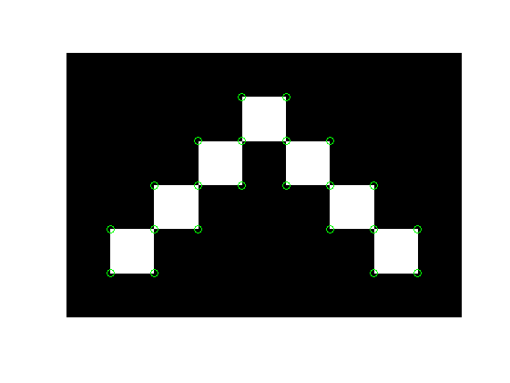
Now I'll graphically illustrate the computational procedure above. First, compute the set of corner locations for all the foreground pixels.
[y,x] = find(bw);
dx = [-0.5 -0.5  0.5  0.5];
dy = [-0.5  0.5 -0.5  0.5];
x_corners = bsxfun(@plus, x, dx);
y_corners = bsxfun(@plus, y, dy);
x_corners = x_corners(:);
y_corners = y_corners(:);
Visualize step 1 by superimposing those corner locations on the input image.
imshow(bw, 'InitialMagnification', 'fit')
hold on
plot(x_corners, y_corners, 'og')
hold off
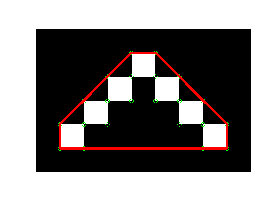
Step 2: Compute the convex hull of all the corner points. Visualize by superimposing the convex hull in red.
k = convhull(x_corners, y_corners);
x_hull = x_corners(k);
y_hull = y_corners(k);
hold on
plot(x_hull, y_hull, 'r', 'LineWidth', 4)
hold off
Step 3: Use poly2mask to convert the convex hull to a binary image mask.
mask = poly2mask(x_hull, y_hull, 6, 9);

imshow(bw, 'InitialMagnification', 'fit')
hold on
h = imshow(mask);
set(h, 'AlphaData', 0.8)
plot(x_hull, y_hull, 'r', 'LineWidth', 4)
hold off
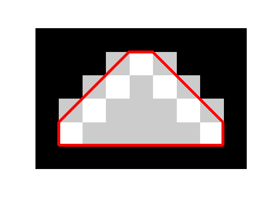
You can see that there are extra pixels along the diagonal edges that got put into the mask. That's not good. If you repeat the operation, those diagonals will keep filling out until you're left with a rectangle. That's not supposed to happen with repeated application of the convex hull.
The reason this is happening is that the convex hull goes exactly through the center of pixels that are along the diagonal but "outside" the original set of foreground pixels. Because of the tie-breaking rules applied by poly2mask, all (in this case) of those outside pixels got included in the output mask.
The solution that I settled on ten years ago, and which is now also used in bwconvhull, was to modify the first step of the procedure. Instead of collecting the set of corner points of each foreground pixel, the correct procedure collects points along the center of each edge of each foreground pixel.
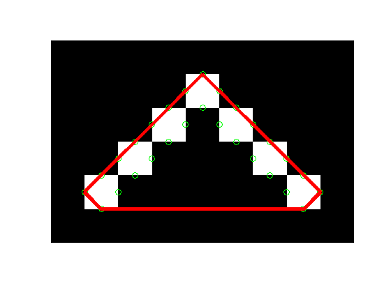
Here's what that looks like.
dx = [0.0  0.0  0.5 -0.5];
dy = [0.5 -0.5  0.0  0.0];
x_edges = bsxfun(@plus, x, dx);
y_edges = bsxfun(@plus, y, dy);
x_edges = x_edges(:);
y_edges = y_edges(:);

k = convhull(x_edges, y_edges);
x_hull = x_edges(k);
y_hull = y_edges(k);

imshow(bw, 'InitialMagnification', 'fit')
hold on
plot(x_edges, y_edges, 'og')
plot(x_hull, y_hull, 'r', 'LineWidth', 4)
hold off
mask = poly2mask(x_hull, y_hull, 6, 9);
imshow(mask, 'InitialMagnification', 'fit')
hold on
plot(x_hull, y_hull, 'r', 'LineWidth', 4)
plot(x_edges, y_edges, 'og')
hold off
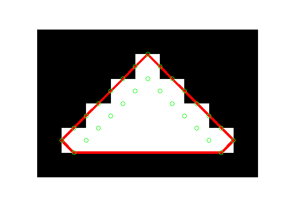
Much better!
I have been fooled more often than I would like to admit by sometimes nonintuitive digital image geometry. For you image processing algorithm people out there, I hope seeing these pictures and techniques will help you avoid similar pitfalls someday.




댓글
댓글을 남기려면 링크 를 클릭하여 MathWorks 계정에 로그인하거나 계정을 새로 만드십시오.