Image binarization – new functional designs
With the very first version of the Image Processing Toolbox, released more than 22 years ago, you could convert a gray-scale image to binary using the function im2bw.
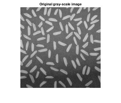
I = imread('rice.png');
imshow(I)
title('Original gray-scale image')

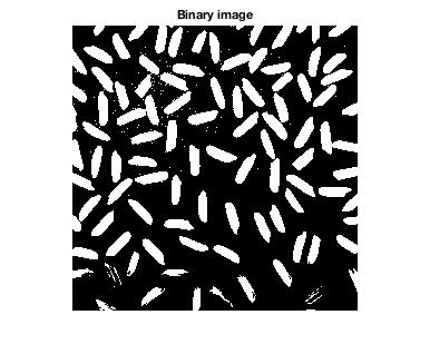
bw = im2bw(I);
imshow(bw)
title('Binary image')

You can think of this as the most fundamental form of image segmentation: separating pixels into two categories (foreground and background).
Aside from the introduction of graythresh in the mid-1990s, this area of the Image Processing Toolbox has stayed quietly unchanged. Now, suddenly, the latest release (R2016a) has introduced an overhaul of binarization. Take a look at the release notes:
imbinarize, otsuthresh, and adaptthresh: Threshold images using global and locally adaptive thresholds
The toolbox includes the new function, imbinarize, that converts grayscale images to binary images using global threshold or a locally adaptive threshold. The toolbox includes two new functions, otsuthresh and adaptthresh, that provide a way to determine the threshold needed to convert a grayscale image into a binary image.
What's up with this? Why were new functions needed?
I want to take advantage of this functionality update to dive into the details of image binarization in a short series of posts. Here's what I have in mind:
- The state of image binarization in the Image Processing Toolbox prior to R2016a. How did it work? What user pains motivated the redesign?
- How binarization works in R2016a
- Otsu's method for computing a global threshold
- Bradley's method for computing an adaptive threshold
Mostly, I haven't written this yet. If there is something particular you'd like to know, tell me in the comments, and I'll try to work it in.


댓글
댓글을 남기려면 링크 를 클릭하여 MathWorks 계정에 로그인하거나 계정을 새로 만드십시오.