One of my favorite aspects of MATLAB for image processing is how I can use a binary image to index directly into a grayscale image. The technique is called logical indexing, and I'm going to show you how it works today.

Note: this is an update of a post I originally wrote in 2008.

Let me start with a small example. (As regular readers know, I like to use magic squares for small matrix examples.)

A = magic(5)

A =

    17    24     1     8    15
    23     5     7    14    16
     4     6    13    20    22
    10    12    19    21     3
    11    18    25     2     9

Every MATLAB user is familiar with ordinary matrix indexing notation.

A(2,3)

ans =

     7

A(2,3) extracts the 2nd row, 3rd column of the matrix A. You can extract more than one row and column at the same time:

A(2:4, 3:5)

ans =

     7    14    16
    13    20    22
    19    21     3

When an indexing expression appears on the left-hand side of the equals sign, that's an assigment. You are changing one or more of the values of the variable on the left-hand side.

A(5,5) = 100

A =

    17    24     1     8    15
    23     5     7    14    16
     4     6    13    20    22
    10    12    19    21     3
    11    18    25     2   100

Here is a frequently-asked MATLAB question: How do I replace all the NaNs in my matrix B with 0s?

An experienced MATLAB user will immediately answer:

B(isnan(B)) = 0;

For example:

B = rand(3,3);
B(2, 2:3) = NaN

B =

    0.2217    0.3188    0.0855
    0.1174       NaN       NaN
    0.2967    0.5079    0.8010

Replace the NaNs with zeros:

B(isnan(B)) = 0

B =

    0.2217    0.3188    0.0855
    0.1174         0         0
    0.2967    0.5079    0.8010

The expression B(isnan(B)) is an example of logical indexing. Logical indexing is a compact and expressive notation that's very useful for many image processing operations.

Let's talk about the basic rules of logical indexing, and then we'll reexamine the expression B(isnan(B)).

If C and D are matrices, then C(D) is a logical indexing expression if D is a logical matrix.

Logical is one of the fundamental data types for MATLAB arrays. Relational operators, such as == or >, produce logical arrays automatically.

C = hilb(4)

C =

    1.0000    0.5000    0.3333    0.2500
    0.5000    0.3333    0.2500    0.2000
    0.3333    0.2500    0.2000    0.1667
    0.2500    0.2000    0.1667    0.1429

D = C > 0.4

D =

  4×4 logical array

   1   1   0   0
   1   0   0   0
   0   0   0   0
   0   0   0   0

If we use D as an index into C with the expression C(D), then we will extract all the values of C corresponding to nonzero values of D and returns them as a column vector. It is equivalent to C(find(D)).

C(D)

ans =

    1.0000
    0.5000
    0.5000

Now we know enough to break down the B(isnan(B)) expression to see how it works.

B = rand(3,3);
B(2, 2:3) = NaN;

nan_locations = isnan(B)

nan_locations =

  3×3 logical array

   0   0   0
   0   1   1
   0   0   0

B(nan_locations)

ans =

   NaN
   NaN

B(nan_locations) = 0

B =

    0.0292    0.4886    0.4588
    0.9289         0         0
    0.7303    0.2373    0.5468

Functions in the Image Processing Toolbox, as well as the MATLAB functions imread and imwrite, follow the convention that logical matrices are treated as binary (black and white) images. For example, when you read a 1-bit image file using imread, it returns a logical matrix:

bw = imread('text.png');
whos bw

  Name        Size             Bytes  Class      Attributes

  bw        256x256            65536  logical              

This convention, together with logical indexing, makes it very convenient and expressive to use binary images as pixel masks for extracting or operating on sets of pixels.

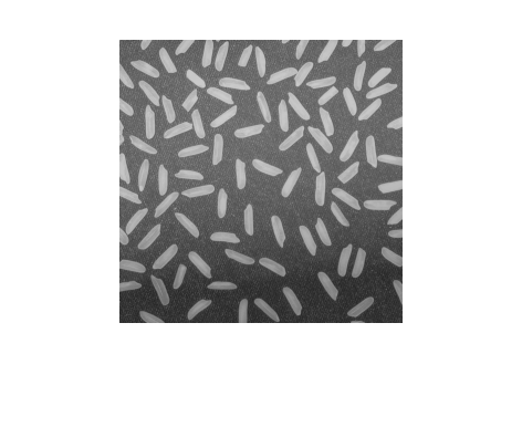
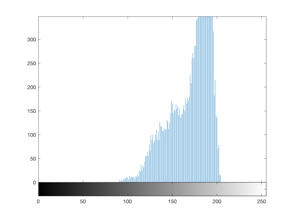
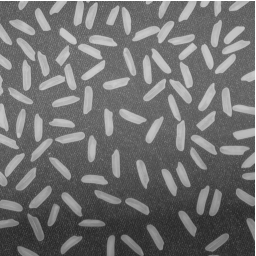
Here's an example showing how to use logical indexing to compute the histogram of a subset of image pixels. Specifically, given a grayscale image and a binary segmentation, compute the histogram of just the foreground pixels in the image.

Here's our original image:

I = imread('rice.png');
imshow(I)

Here's a segmentation result (computed and saved earlier), represented as a binary image:

url = 'https://blogs.mathworks.com/images/steve/192/rice_bw.png';
bw = imread(url);
imshow(bw)

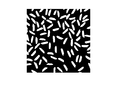
Now use the segmentation result as a logical index into the original image to extract the foreground pixel values.

foreground_pixels = I(bw);
whos foreground_pixels

  Name                       Size            Bytes  Class    Attributes

  foreground_pixels      17597x1             17597  uint8              

Finally, compute the histogram of the foreground pixels.

figure
imhist(foreground_pixels)

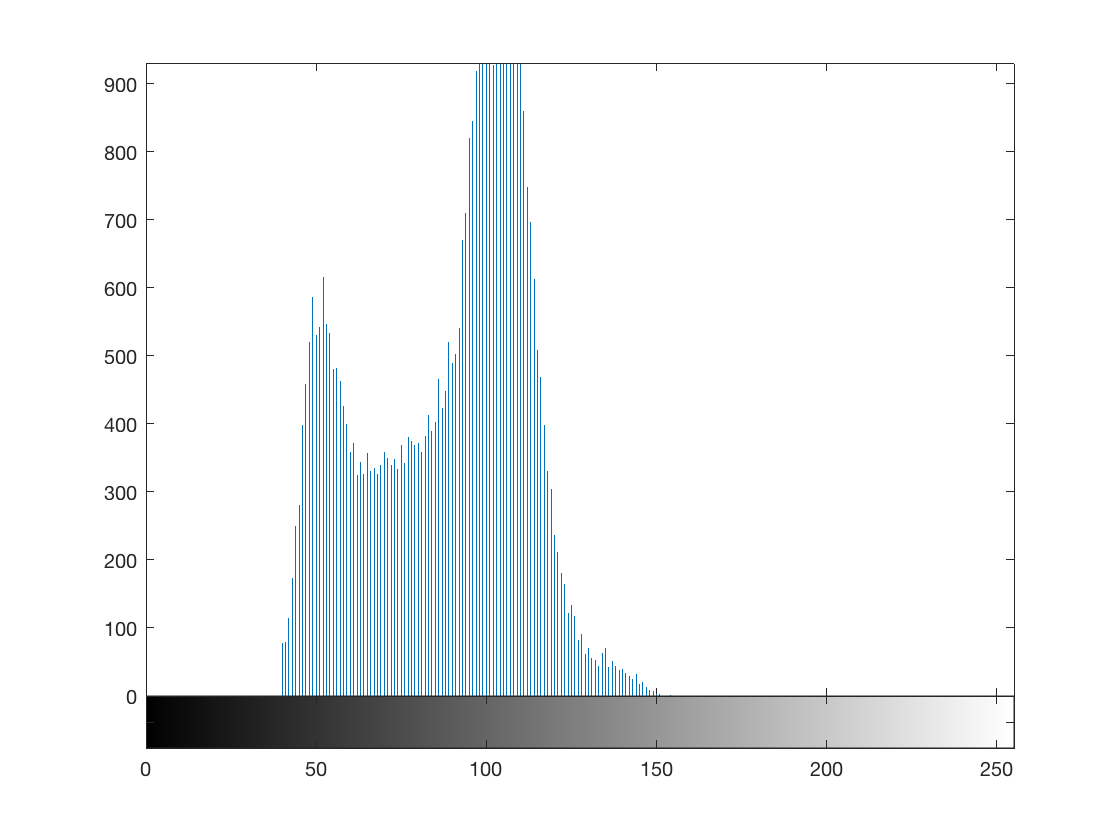
As another example, you could complement the binary image to compute something based on the background pixels.

imhist(I(~bw))

PS. I expect that this will be the last blog post that I write using R2016b. Keep an eye on the downloads page!

Get the MATLAB code

Published with MATLAB® R2016b