
Mastering Autonomous Parking using Simulink and ROS
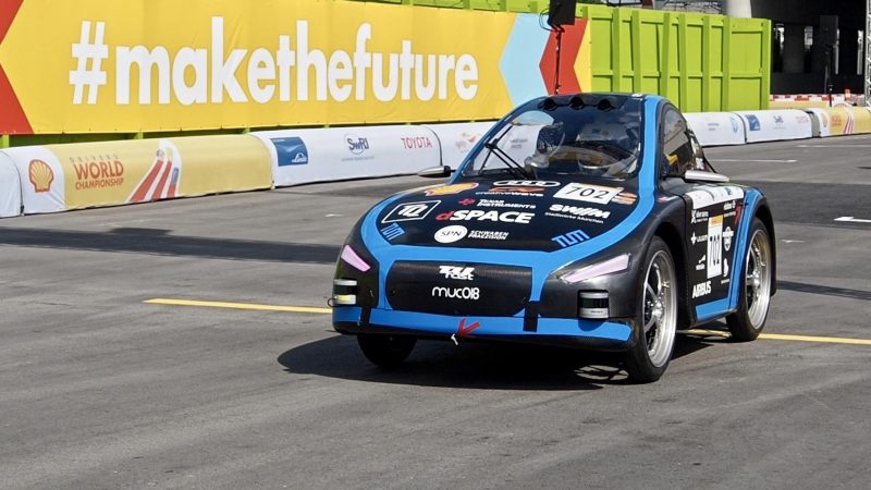
Today’s guest post is by Maximilian Mühlbauer. Maximilian was head of autonomous driving at TUfast Eco for the last season and will share their autonomous journey for the 2018 Shell Eco-marathon Autonomous UrbanConcept challenge.
—
Back in 2016, we started developing a speed controller to assist the driver in our efficiency challenges which proved to be very helpful. The optimization in the back-end and the controller were already presented in a Racing Lounge video “Cruise Control in Efficiency Challenges”.
For our endeavor in 2018, we took the next big step and developed a fully autonomous system. Our goal was to build a fully integrated vehicle one would love to take for daily life. To demonstrate our approach, we will take a closer look at the parking challenge.

Figure Task is to park in the marked rectangle as close to the blue block as possible
Hardware Setup and Software Architecture
The electrical components used in our cars so far were based on microcontrollers and low-power sensors consuming less power than your smartphone to maximize efficiency. For driving completely autonomously, we clearly needed more power and state-of-the-art sensors.
Two Lidar sensors form the heart of our perception system as the main challenge is detecting track boundaries and physical objects. A wide-angle mono camera for object detection and a stereo camera for depth perception are installed to classify objects. For instance, the mono camera was used to clearly distinguish the parking block from the track boundaries. Ultrasonic sensors complement the setup – they allow us to correctly estimate small distances and so to maneuver as close as five centimeters to the parking block.
Video Sensor of muc18: Lidars, mono + stereo cameras, ultrasonic sensors
For the perception part, we used an NVIDIA DRIVE™ PX2 which is sufficiently powered to handle complex processing tasks. It can also be targeted using the GPU Coder™, which we’ve done with our occupancy grid inflation algorithm. For our planning and control system, we relied on the dSPACE MicroAutoBox II with Embedded PC. This box includes a real-time target for Simulink to run our control algorithms and a standard PC to run the planning algorithms.
Our software system is based on ROS. It allows us to distribute our software over various computers and to use readily available drivers. We aim for a highly modularized system to be able to easily replace and test components.

Figure Software architecture
The environmental model primarily consists of an occupancy grid in which free space for driving is determined. Object detection is mainly relying on camera data. The algorithms used benefit massively from GPU support.
The high-level and trajectory planning run on the Embedded PC. State estimation and control algorithms run on the real-time µAutoBox. All parts were designed to efficiently use computational resources to keep enough power to allow further developments.
One point in which our setup greatly differs from other systems is that we don’t use a pre-built map. One reason for this is because we feel that an autonomous car should be able to fully replace a human driver – and a human driver only has the surroundings of the car which it can see as input. We wanted to replicate the dependency on live data from the car’s sensors. Our system should be able to navigate in previously unknown areas – just like autonomous cars will have to in complex, ever-changing urban environments. This leads to “probabilistic” approaches for goal point and trajectory generation. We had to weigh in different factors to find the best possible solution for the planning problem, without exactly knowing where to go.
Simulation-Driven Development
Our major goal was to perform a closed-loop simulation of all components. This was needed because the car was yet to be built. Additionally, an autonomous system like we’ve built it, with complex and time-critical interaction between perception, planning and control is too complex to be tested on prototype hardware only.
We chose a two-fold approach: One simulation for the perception and planning part and one simulation for our control algorithms. This way, we could significantly reduce complexity and computational power needed to run the simulations.
The control simulation worked in a straightforward manner, we replaced real inputs and outputs in our simulation by a model of the car. This was the two-track model used for our efficiency simulation, extended by the vehicle’s internal states that we needed for the logic of the autonomous system. We could then use pre-defined trajectories to validate our control algorithms.
Using trajectories that inlcude time information together with the geometrical path was an important concept decision. They are not needed for the type of challenges to be performed in the autonomous competition. However, to drive in a dynamic environment, they are necessary. Collision-checking in such an environment is not feasible for a static-path solution. Rather, it requires real-time information about the exact location at all times.

Figure Components of a trajectory with safe stop
For generating perception input, we relied on Gazebo, which can simulate various sensors and export the output directly to ROS topics. For moving the car, we developed a plugin, which would execute the calculated trajectories. This closed-loop simulation was especially important for us because dynamic perception and planning is more difficult than optimizing an algorithm on static scenes.
In the figure below, you can see how we developed our planning algorithm. Input for the planning algorithm is an inflated occupancy grid, the previous trajectory and a goal point. The occupancy grid is inflated via Minkowski dilatation with a circle specific to the challenge. The algorithm is programmed in MATLAB and then exported to run on the GPU with GPU Coder™.

Figure The path underlying the above trajectory
The planning algorithm then calculates a set of possible goal positions around the goal point and connects them to the start via polynomials. Feasible paths are then evaluated using different metrics, e.g. curvature and possible collision on the Occupancy Grid. Non-admissible paths are shown in red, the curvature-optimal path is drawn in yellow and the finally selected trajectory is drawn in green.
We’ve developed a script to take the input from ROS, do the calculation and then display the generated path and trajectory. This way, we could look under the hood of our planning algorithm and see what it would plan to do in specific positions. For running on the car, the algorithm is of course exported to C++ code and compiled.
One of the most challenging aspects, however, is to find the target point as we don’t have a map of the track. In track-following operation mode, we used an extended version of the ray-casting algorithm to find out where we could see furthest forward in the occupancy grid. This point was then used as target point. The most important aspect here is to find a good weight factor which could deal with inaccurate measurements. We used the simulation to find the best values for that. Here, the implementation as a Simulink ROS node helped us greatly: we could directly debug our algorithm and change values during simulation.
To do this, we needed to slow down the simulation to ROS time as the simulation is advancing slower than real-time. This can be done by obtaining the ROS time in Simulink via the ROS Time block and then slowing down the simulation with code similar to the Real-Time Pacer. We did also integrate the tf transformation tree by using interpreted MATLAB code during simulation time to access the rostf object.
Once the car has spotted and localized the parking block, the optimal parking position behind the parking block was used as goal point. From this moment on, the car drives a S-shaped path to the parking box. This can be seen in the below video of the simulation.
Video Autonomous parking in simulation
The left view shows how the car moves in the simulation environment on the top. The left bottom shows the view from the front camera overlaid with the perception of the start lines and the parking block. On the right side, the rviz view of the scene is displayed. It includes the car location and the occupancy grid together with the perceived parking block (red, big dot). The target points (green line) as well as the planned trajectory (orange) and the full-length path (blue) are also included. The full-length path sometimes disappears because we plan for the future and rviz then isn’t able to do the tf transform.
Deployment and Testing
When the algorithms were mature enough, we started testing on the real hardware. The real-time unit could be directly flashed from our notebooks. For the rest, we cloned the repositories and built the software directly on the target hardware.
For our Simulink ROS nodes, we also needed to integrate with the ROS time. This can now be easily done when checking “enable ROS time stepping”. For accessing the tf tree, a bit more work needs to be done: we essentially had to write our subscriber C++ code which we could then be called from a MATLAB function. Of course, the “tf” dependency has to be added to the package.xml and the CMakeList-file.
One of the biggest issues on the real hardware was to get an accurate timing for the trajectories to be executed properly. We synchronized the involved machines using the network time (ntp) protocol. The real-time unit was synced using high-priority CAN messages. We also had to remove additional delays introduced in our models to support a low-latency operation. Only after doing this, we achieved a smooth motion of the car.
After these things were solved, the planning system remained a big problem. We initially had an approach that considered hard “occupied” vs. “not occupied” thresholds on the occupancy grid. While this worked well with the precise sensor readings in simulation, it didn’t quite work in reality. With sensor distortions e.g. coming from bumps in the road, this approach would eventually fail to find a feasible path. One other concern was the ‘being trapped’-case in an inflated obstacle, where the initial algorithm wouldn’t find a way out.
We then stepped back into the simulation to develop the more probabilistic approach, giving occupancy values only a weight. Once we found a good initial setup, we returned to the test track to fine-tune the values. We regularly stopped in positions where the algorithm previously failed and checked directly in MATLAB how we could overcome the issue. In the end, this allowed us to develop the whole planning system with quite a few iterations in a very short time. In fact, the system we finally used at the competition was developed, including testing, in just four weeks. The system proved to work well at the competition.
Another issue related to imperfections in real-world comes when trying to park as close to the parking block as possible. During the simulation, we get very accurate readings for all the sensors and we perfectly know our position. In reality, this is much more difficult to achieve. Therefore, we relied on ultrasonic sensors for close ranges and implemented a switch from trajectory-following to position control once the parking block was sensed directly ahead. This had to be tuned on the real car because the stopping behavior depends greatly on the braking behavior, which couldn’t be fully modeled.
The ultimate testing, however, is performed at the competition. New challenges arrived like parking down-hill which we’ve never tried out before. This requires much more braking power and an earlier stopping than we needed during testing. Therefore, we had to tune the parameters again to successfully complete the challenge.
Conclusion
In just one year’s time, we’ve built a successful autonomous car. Of course, this has several drawbacks over refitting an existing car – the most severe being that we were only able to test shortly before the competition. However, it allowed us to build a car with autonomy in mind. We’ve learnt what is important and we could contribute our vision for the autonomous mobility of the future with muc018.


评论
要发表评论,请点击 此处 登录到您的 MathWorks 帐户或创建一个新帐户。