Mitigating Climate Change through Deep Learning in MATLAB

作者 Tanya Kuruvilla, March 27, 2023

9 次查看（过去 30 天） | 0 个赞 | 0 个评论

Joining us today is Kaveh Faraji and Azin Al Kajbaf, who won the Best Use of MATLAB award for The BioMassters competition! Read on to learn more about this duo and how they used deep learning for biomass estimation. Over to you guys…

Azin got her Ph.D. in Civil Engineering from the University of Maryland in 2022 and is currently a postdoctoral research fellow at Johns Hopkins University and the National Institute of Standards and Technology (NIST). Kaveh is a Ph.D. candidate in Civil Engineering at the University of Maryland. Our area of academic focus involves the application of machine learning, geospatial analysis, and statistical methods in natural hazard assessment. We started to use deep learning a few years ago. We were implementing machine learning for our research at the time using MATLAB and were also interested in deep learning. MathWorks was sponsoring a deep learning competition at the time, which motivated us to learn about MATLAB’s Deep Learning Toolbox and deep learning concepts in general. Since then, we have participated in multiple deep learning competitions. Currently, we are working on research projects involving machine learning and deep learning applications in the assessment of natural hazards. We have been planning to get some hands-on experience in the application of machine learning and deep learning in working with satellite imagery, which could ultimately be helpful in our research too, and this specific competition provided us with the perfect opportunity.

Inspiration

We are a postdoctoral researcher and a Ph.D. student. We implement machine learning and deep learning methods in our research projects, and MATLAB is one of the programming languages that we use. Participating in data science competitions has become our passion since it motivates us to learn more about machine learning and deep learning methods and their real-world applications. The BioMassters competition was particularly interesting because we recently started to work with satellite imagery for natural hazard assessment in our research.

Breaking down the problem

The satellite imagery data contains 15 bands (11 bands for Sentinel-2 and 4 bands for Sentinel-1) for 12 months. The objective was to predict the yearly biomass of these images (pixel values of labels). The data has spatial and temporal aspects. Our idea was:

Perform pixel-by-pixel classification of images without considering the spatial effects (for this, we used 1-D CNN)
Then use a 3-D U-Net structure to consider the spatial relationship between pixels.

How did we implement it?

This solution contains two main steps:

Step 1: Pixel-by-pixel regression with a 1-D CNN

In this network, we read each image and used a custom training loop for training the network. We reshaped satellite imagery (with the size of [15 * 12 * 256 * 256]) to a matrix with the shape of [channel_size(C) = 15 batch_size(B) = (256*256) temporal_size(T) = 12]. We predicted labels for each image in training and testing datasets.

For example, you can see the code below, which we used to create and train a 1-D CNN that improved the score.

%% Buidling a 1-D CNN

filterSize = 3;

numFilters = 64;

numClasses=10;

layers = [ …

 sequenceInputLayer(15, MinLength=12)

 convolution1dLayer(filterSize,numFilters,Padding=“causal”)

 reluLayer

 layerNormalizationLayer

 maxPooling1dLayer(2)

 convolution1dLayer(filterSize,2*numFilters,Padding=“causal”)

 reluLayer

 layerNormalizationLayer

 globalMaxPooling1dLayer

 fullyConnectedLayer(512)

 reluLayer

 fullyConnectedLayer(128)

 reluLayer

 fullyConnectedLayer(1)

 reluLayer];

% analyzeNetwork(layers);

lgraph = layerGraph(layers);

net = dlnetwork(lgraph);

%% Using the pre-trained model or training the model

% If you want to train the model from scratch, change “train_network” value

% to true.

train_network = true;

if train_network

 miniBatchSize = 1;

 numEpochs = 10;

 numObservations = numel(inputTrain.Files);

 numIterationsPerEpoch = floor(numObservations./miniBatchSize);

 averageGrad = [];

 averageSqGrad = [];

 numIterations = numEpochs * numIterationsPerEpoch;

 monitor = trainingProgressMonitor(Metrics=“Loss”,Info=“Epoch”,XLabel=“Iteration”);

 iteration = 0;

 epoch = 0;

 while epoch < numEpochs && ~monitor.Stop

 epoch = epoch + 1;

 % Shuffle data.

 shuffle(mbq);

 reset(mbq_val);

 while hasdata(mbq) && ~monitor.Stop

 iteration = iteration + 1;

 % Read mini-batch of data.

 [X,T] = next(mbq);

 % Convert mini-batch of data to a dlarray.

 X = dlarray(single(X),“CBT”);

 % We read each image with the size of [15 * 12 * 256 * 256] and

 % convert it to a [channel_size(C) = 15 batch_size(B) = (256*256) temporal_size(T) = 12]

 % We had to use a batch size smaller than 65501.

 % We got errors when we used batch size above this value.

 X = X(:,1:65500,:);

 T = T(:,1:65500,:);

 % If training on a GPU, then convert data to a gpuArray.

 if canUseGPU

 X = gpuArray(X);

 T= gpuArray(T);

end

 % Calculate loss and gradients using the helper loss function.

 [loss,gradients] = dlfeval(@modelLoss,net,X,T);

 % Update the network parameters using the Adam optimizer.

 [net,averageGrad,averageSqGrad] = adamupdate(net,gradients,averageGrad,averageSqGrad,iteration);

 % Update the training progress monitor.

 recordMetrics(monitor,iteration,Loss=loss);

 updateInfo(monitor,Epoch=epoch + ” of ” + numEpochs);

 monitor.Progress = 100 * iteration/numIterations;

end

 % Validation error

 ii=0;

 while hasdata(mbq_val)

 [X_val, T_val]= next(mbq_val);

 if canUseGPU

 X_val = dlarray(single(X_val),“CBT”);

 T_val = gpuArray(T_val);

end

 Y_val = predict(net,X_val);

 error = mse(Y_val, T_val)^.5;

 ii=ii+1;

 rmse_error(ii) = extractdata(gather(error));

 % disp(rmse_error(ii))

end

 disp([‘Epoch’+ string(epoch)+‘ Validation Error(RMSE): ‘ , mean(rmse_error)])

end

 save(‘trainedNetwork_conv1d_submit.mat’,‘net’)

else

 lgraph = load(‘trainedNetwork_conv1d.mat’);% Load pre-trained network

 net = lgraph.net;

end

Step 2: Using a 3-D U-Net Model

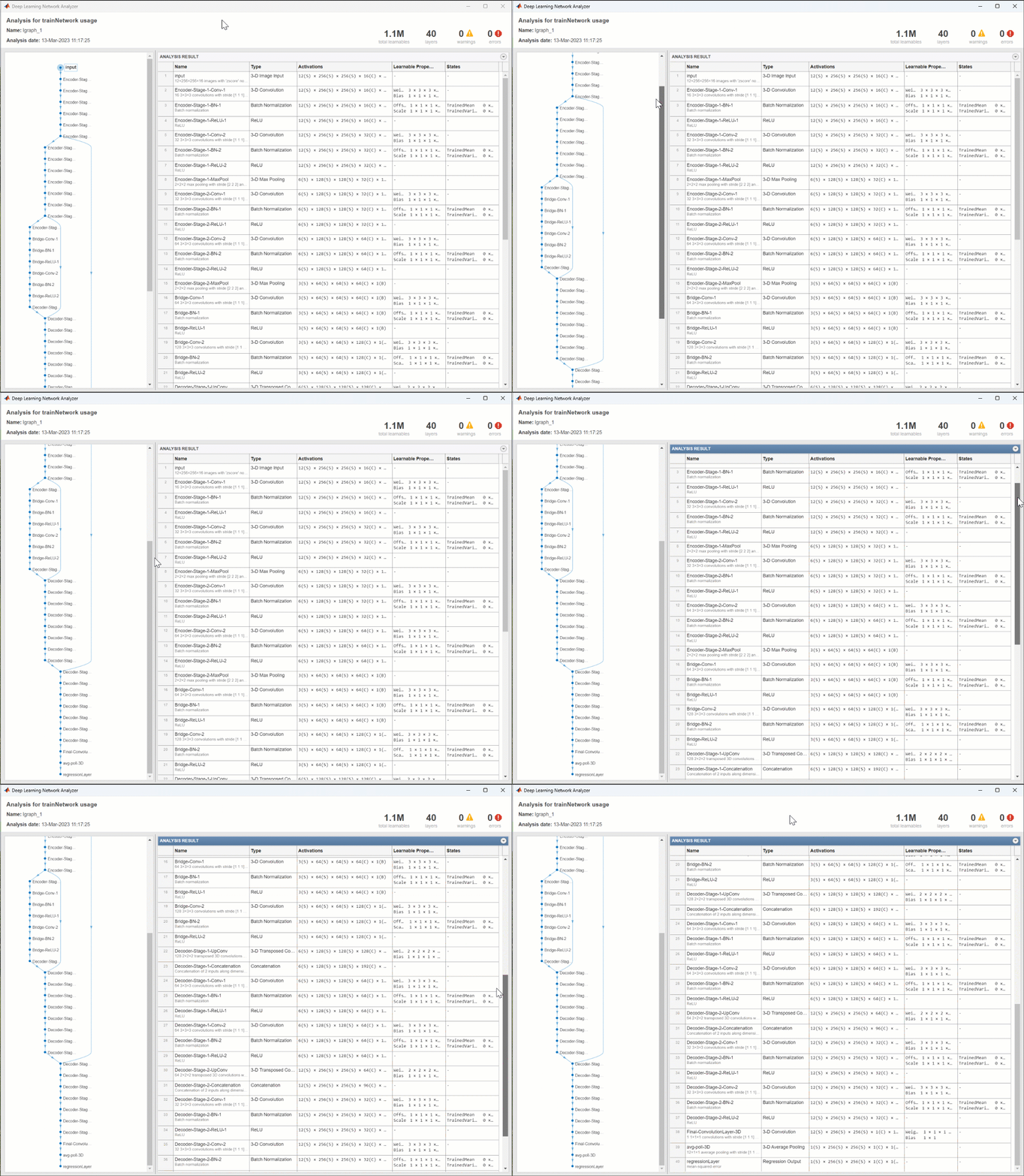
Next, we used a 3-D U-Net model and provided it with inputs with the shape of [16*12*256*256]. The 16th channel in the input of the U-Net network is the labels generated in step 1. You can see more details about this model in the GIF below:

Results

In the below figure, you can see a summary of our solution’s framework and the final score.

Key Takeaways

This competition provided us with the opportunity to employ deep learning in a new area. We figured that for a project of this nature with the purpose of assigning values or labels to satellite imagery pixels, an ensemble model is required to achieve better performance. The ensemble could include a model that performs pixel-by-pixel prediction and a model that considers the effect of surrounding pixels (3D U-net). We also would like to highlight our experience working with MATLAB’s custom network training loop, which was flexible and intuitive. We had experience working with MATLAB toolboxes in our previous projects. We find the MATLAB Deep Learning Toolbox user-friendly, and most of the time we can find a solution to our problems using documentation and MATLAB Answers.

We want to thank MathWorks for sponsoring this competition. It provided a great opportunity to get hands-on experience working with satellite imagery with spatial and temporal aspects and learn more about MATLAB’s Deep Learning Toolbox capabilities.

Run in your browser