Steve on Image Processing

I described in my previous connected component labeling post the algorithm used by bwlabeln. This time I'll talk about the variation used by bwlabel. This variation uses run-length encoding as the first step.

Here's what I mean by run-length encoding. Consider this small binary image matrix:

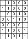
Such a binary image can be represented as a collection of runs, or sequences of 1s. Working columnwise, this image contains 9 runs:

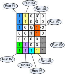
Each run can be represented by its starting pixel and by the number of pixels in the run, which is called the run length. Hence the term run-length encoding.

For a larger binary image containing larger objects, the number of runs can be much smaller than the number of foreground pixels. But the connectivity analysis can be completely determined based on the runs. In our small example:

This set of connectivity pairs can be resolved into equivalence classes using the technique I described earlier based on dmperm. In this example there are only two equivalence classes, corresponding to the two connected components.

The function bwlabel calls computes a run-length encoding first. As it finds each run, it also determines which runs on the previous column are connected, if any. Then it constructs a sparse adjacency matrix and calls dmperm to compute the equivalence classes. Then it labels each run in the output label matrix according to the equivalence class it belongs to.

This is a very efficient method because it scans each pixel in the input image only once, and also because the adjacency matrix is usually relatively small. It is R-by-R, where R is the number of runs.

You can find this method described in Haralick and Shapiro, Computer and Robot Vision Volume 1, Addison-Wesley, 1992, pp. 40-48. (Note that the equivalence class resolution method used by bwlabel is different than the one described in the book.)

Get the MATLAB code

Published with MATLAB® 7.4