
Image deblurring – Wiener filter
I'd like to welcome back guest blogger Stan Reeves, professor of Electrical and Computer Engineering at Auburn University. Stan will be writing a few blogs here about image deblurring.
In my last blog, I looked at image deblurring using an inverse filter and some variations. The inverse filter does a terrible job due to the fact that it divides in the frequency domain by numbers that are very small, which amplifies any observation noise in the image. In this blog, I'll look at a better approach, based on the Wiener filter.
I will continue to assume a shift-invariant blur model with independent additive noise, which is given by
y(m,n) = h(m,n)*x(m,n) + u(m,n)
where * is 2-D convolution, h(m,n) is the point-spread function (PSF), f(m,n) is the original image, and u(m,n) is noise.
The Wiener filter can be understood better in the frequency domain. Suppose we want to design a frequency-domain filter G(k,l) so that the restored image is given by
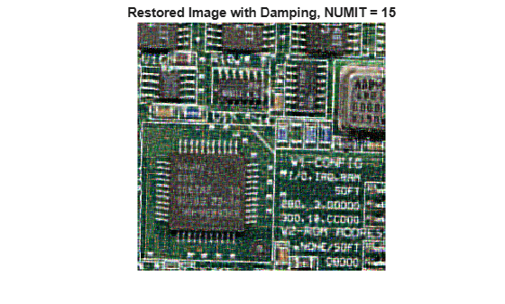
We can choose G(k,l) so that we minimize

E[] is the expected value of the expression. We assume that both the noise and the signal are random processes and are independent of one another. The minimizer of this expression is given by


This filter gives the minimum mean-square error estimate of X(k,l). Now that sounds really great until we realize that we must supply the signal and noise power spectra (or equivalently the autocorrelation functions of the signal and noise).
The noise power spectrum is fairly easy. We usually assume white noise, which makes the noise power spectrum a constant. But how do we determine what this constant is? If

then the noise power spectrum is given by
for an MxN image. This noise variance may be known based on knowledge of the image acquisition process or may be estimated from the local variance of a smooth region of the image.
The signal power spectrum is a little more challenging in principle, since it is not flat. However, we have two factors working in our favor: 1) most images have fairly similar power spectra, and 2) the Wiener filter is insensitive to small variations in the signal power spectrum.
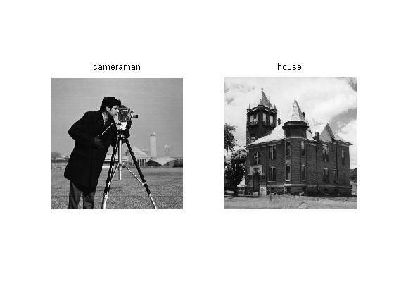
Consider two very different images -- the cameraman and house.
cam = im2double(imread('cameraman.tif'));
house_url = 'https://blogs.mathworks.com/images/steve/180/house.tif';
house = im2double(imread(house_url));

subplot(1,2,1)
imshow(cam)
colormap(gray(256))
title('cameraman')
subplot(1,2,2)
imshow(house)
title('house')
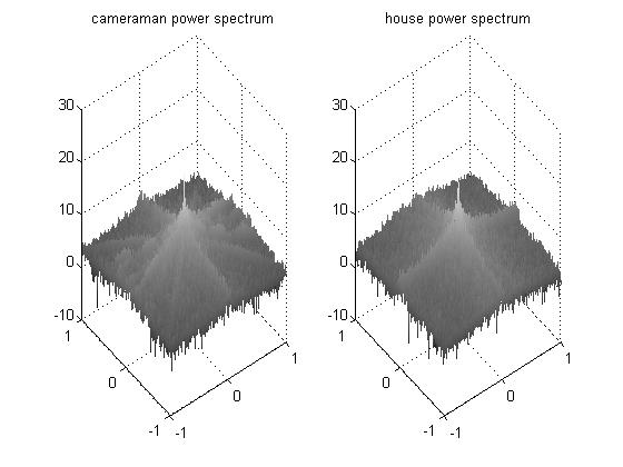
We show the actual (log) spectrum for these two images.
cf = abs(fft2(cam)).^2;
hf = abs(fft2(house)).^2;
subplot(1,2,1)
surf([-127:128]/128,[-127:128]/128,log(fftshift(cf)+1e-6))
shading interp, colormap gray
title('cameraman power spectrum')
subplot(1,2,2)
surf([-127:128]/128,[-127:128]/128,log(fftshift(hf)+1e-6))
shading interp, colormap gray
title('house power spectrum')
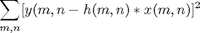
Let's see what happens if we restore the cameraman with the actual power spectrum.
h = fspecial('disk',4);
cam_blur = imfilter(cam,h,'circular');
% 40 dB PSNR
sigma_u = 10^(-40/20)*abs(1-0);
cam_blur_noise = cam_blur + sigma_u*randn(size(cam_blur));

cam_wnr = deconvwnr(cam_blur_noise,h,numel(cam)*sigma_u^2./cf);
subplot(1,1,1)
imshow(cam_wnr)
colormap(gray(256))
title('restored image with exact spectrum')

For comparison purposes, we restore the cameraman using the power spectrum obtained from the house image.
cam_wnr2 = deconvwnr(cam_blur_noise,h,numel(cam)*sigma_u^2./hf);
imshow(cam_wnr2)
colormap(gray(256))
title('restored image with house spectrum')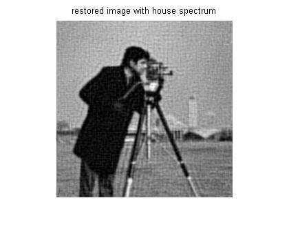
Visually, the two are very similar in quality. In terms of mean-square error (MSE), the former is better (lower), as the theory predicts:
format short e
mse1 = mean((cam(:)-cam_wnr(:)).^2)
mse2 = mean((cam(:)-cam_wnr2(:)).^2)
mse1 =

  2.9905e-003


mse2 =

  3.9191e-003
In both cases, the spectrum is concentrated in the low frequencies and falls away at higher frequencies. A smoothed version of the spectra would look even more similar. Rather than using the power spectrum from a specific image, one can either average a large number of images or use a simple model of the power spectrum or autocorrelation function.
A common model for the image autocorrelation function is
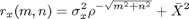


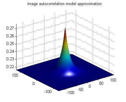
We calculate these parameters for the cameraman, averaging over horizontal and vertical shifts to get a single parameter for the correlation coefficient. Then we calculate an autocorrelation function.
sigma2_x = var(cam(:))
mean_x = mean(cam(:))
cam_r = circshift(cam,[1 0]);
cam_c = circshift(cam,[0 1]);
rho_mat = corrcoef([cam(:); cam(:)],[cam_r(:); cam_c(:)])
rho = rho_mat(1,2);
[rr,cc] = ndgrid([-128:127],[-128:127]);
r_x = sigma2_x*rho.^sqrt(rr.^2+cc.^2) + mean_x^2;

surf([-128:127],[-128:127],r_x)
axis tight
shading interp, camlight, colormap jet
title('image autocorrelation model approximation')
sigma2_x =

  5.9769e-002


mean_x =

  4.6559e-001


rho_mat =

  1.0000e+000  9.4492e-001
  9.4492e-001  1.0000e+000
From this we calculate another restored image:
cam_wnr3 = deconvwnr(cam_blur_noise,h,sigma_u^2,r_x);
imshow(cam_wnr3)
colormap(gray(256))
title('restored image using correlation model')
mse3 = mean((cam(:)-cam_wnr3(:)).^2)
mse3 = 3.5255e-003

The restored image from this method is better than the restored image using the house spectrum but not quite as good as the one using the exact cameraman spectrum. All in all, we can see that the exact noise-to-signal spectrum isn't necessary to yield good results.
- by Stan Reeves, Department of Electrical and Computer Engineering, Auburn University
- Category:
- Image deblurring


Comments
To leave a comment, please click here to sign in to your MathWorks Account or create a new one.