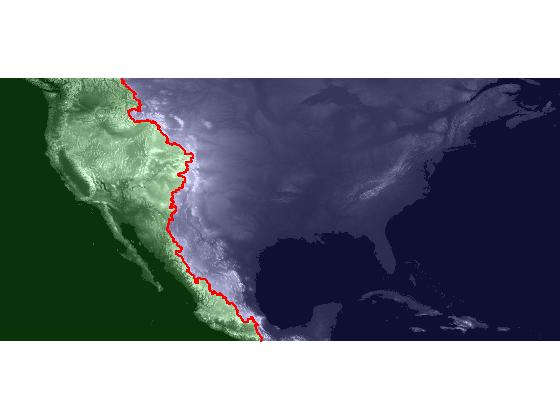
Locating the US continental divide, part 2 – Watershed transform

Posted by Steve Eddins, May 1, 2009

6 views (last 30 days) | 0 Likes | 1 comment

This post is the second in my series on computing the location of the US continental divide. Today I'm going to look at the watershed transform, including how to compute and visualize it using the Image Processing Toolbox functions watershed and label2rgb.

The watershed transform of an image treats image pixel values as surface heights. It divides image pixels into catchment basins, a term borrowed from geography. A catchment basin is the geographical area draining into a river or reservoir. A watershed ridge divides catchment basins.

The function watershed identifies catchment basins and ridge pixels in an image. Let me illustrate with a one-dimensional example.

H = [4 3 2 3 6 7 5 4 3 3]

H =

     4     3     2     3     6     7     5     4     3     3

L = watershed(H)

L =

     1     1     1     1     1     0     2     2     2     2

The output of watershed is telling us that there are two catchment basins in H, corresponding to the elements of L equal to 1 and 2. The element of L equal to 0 corresponds to the element of H equal to 7; this element is a local maximum that sits between two catchment basins. It is called a ridge pixel. We call L a label matrix. The toolbox functions watershed, bwlabel, and bwdist all produce output in this form.

Normally in image processing, the watershed transform is used in situations where the pixel values do not literally represent height values. (See my MATLAB News & Notes article on using the watershed transform for image segmentation.)

For this series, though, we really do have an image whose pixel values represent height, and the watershed transform is what we want to use to compute the continental divide. Essentially, we're looking for the Pacific Ocean and Atlantic Ocean catchment basins for the continental US.

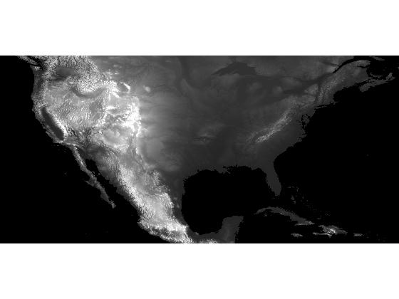
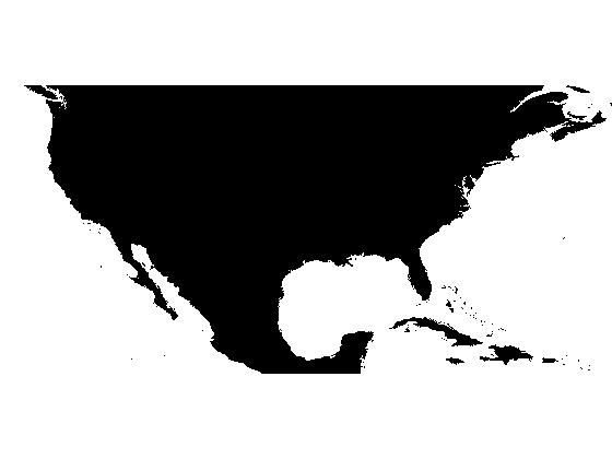
So let's try computing the watershed transform of our DEM (digital elevation model). I saved the DEM to a MAT-file in my previous post in this series.

s = load('continental_divide');
dem = s.dem_cropped;
display_range = [-500 3000];
imshow(dem, display_range, 'InitialMagnification', 'fit');

L = watershed(dem);

The toolbox function label2rgb is useful for visualizing label matrices. It converts a label matrix to an image, with different colors assigned to the different catchment basins. I'll use label2rgb to visualize L using the jet colormap, with ridge pixels displayed as white and catchment basin colors assigned randomly.

rgb = label2rgb(L, 'jet', 'w', 'shuffle');
imshow(rgb, 'InitialMagnification', 'fit')

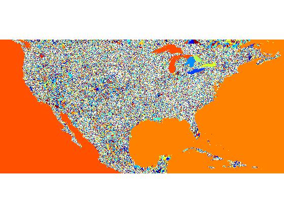
Oh boy, what a mess! What does that even mean? Let's zoom in much closer to see what's really going on.

axis([5580 5670 2060 2100])

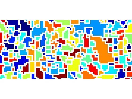
It looks we have a very large number of catchment basins, most of which contain only a few pixels. How many catchment basins are there? Just look at the maximum value of L.

max(L(:))

ans =

      540976

So there are more than half a million distinct catchment basins detected by watershed.

The next posts in this series will examine why there are so many, and how to get down to just two.

About this Series

This series explores the problem of computing the location of the continental divide for the United States. The divide separates the Atlantic and Pacific Ocean catchment basins for the North American continent.

As an algorithm development problem, computing the divide lets us explore aspects of data import and visualization, manipulating binary image masks, label matrices, regional minima, and the watershed transform.

Part 1 - Introduction. Data import and display. multibandread, imshow.

Part 2 - Watershed transform. watershed, label2rgb.

Part 3 - Regional minima. imerode, imregionalmin.

Part 4 - Ocean masks. binary image manipulation, bwselect.

Part 5 - Minima imposition. imimposemin.

Part 6 - Computing and visualizing the divide. watershed, label2rgb, bwboundaries.

Part 7 - Putting it all together. One script that does everything, from data import through computation and visualization of the divide.

Data credit: GLOBE Task Team and others (Hastings, David A., Paula K. Dunbar, Gerald M. Elphingstone, Mark Bootz, Hiroshi Murakami, Hiroshi Maruyama, Hiroshi Masaharu, Peter Holland, John Payne, Nevin A. Bryant, Thomas L. Logan, J.-P. Muller, Gunter Schreier, and John S. MacDonald), eds., 1999. The Global Land One-kilometer Base Elevation (GLOBE) Digital Elevation Model, Version 1.0. National Oceanic and Atmospheric Administration, National Geophysical Data Center, 325 Broadway, Boulder, Colorado 80305-3328, U.S.A. Digital data base on the World Wide Web (URL: http://www.ngdc.noaa.gov/mgg/topo/globe.html) and CD-ROMs.

Published with MATLAB® 7.8