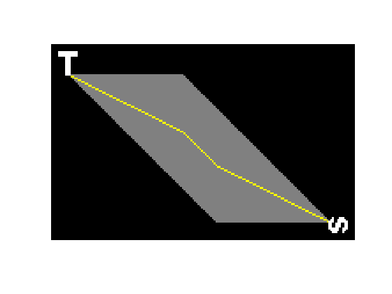
In this post in the Exploring shortest paths series, I make things a little more complicated (and interesting) by adding constraints to the shortest path problem. Last time, I showed this example of finding the shortest paths between the "T" and the sideways "s" in this image:

url = 'https://blogs.mathworks.com/images/steve/2011/two-letters-cropped.png';
bw = imread(url);

And this was the result:

What if we complicate the problem by adding other objects to the image and looking for the shortest path that avoids these other objects?

For example, what if we want to find a shortest path between the "T" and the sideways "s" without going through any of other letters between them in the image below?

url = 'https://blogs.mathworks.com/images/steve/2011/text-cropped.png';
text = imread(url);
imshow(text, 'InitialMagnification', 'fit')

We can do this by using bwdistgeodesic instead of bwdist in our algorithm. bwdistgeodesic is a new function in the R2011b release of the Image Processing Toolbox. In addition to taking a binary image input that bwdist takes, it takes another argument that specifies which pixels the paths are allowed to traverse.

Let's use our text image to make a mask of allowed path pixels.

mask = ~text | bw;
imshow(mask, 'InitialMagnification', 'fit')

Next, we make our two binary object images as before.

L = bwlabel(bw);
bw1 = (L == 1);
bw2 = (L == 2);

Next, instead of using bwdist, we use bwdistgeodesic.

D1 = bwdistgeodesic(mask, bw1, 'quasi-euclidean');
D2 = bwdistgeodesic(mask, bw2, 'quasi-euclidean');

D = D1 + D2;
D = round(D * 8) / 8;

D(isnan(D)) = inf;
paths = imregionalmin(D);

paths_thinned_many = bwmorph(paths, 'thin', inf);
P = false(size(bw));
P = imoverlay(P, ~mask, [1 0 0]);
P = imoverlay(P, paths, [.5 .5 .5]);
P = imoverlay(P, paths_thinned_many, [1 1 0]);
P = imoverlay(P, bw, [1 1 1]);
imshow(P, 'InitialMagnification', 'fit')

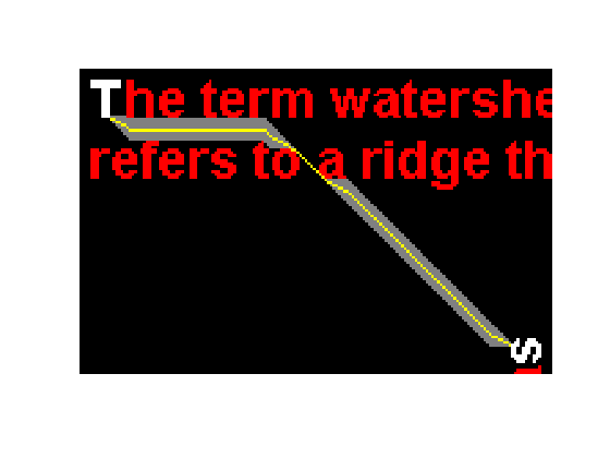
In the image above, the white characters are the starting and ending points for the path. The path is not allowed to pass through the red characters. The gray pixels are all the pixels on any shortest path, and the yellow pixels lie along one particular shortest path.

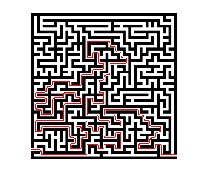
Let's have a little fun by using this technique to solve a maze. Here's a test maze (created by The Maze Generator).

url = 'https://blogs.mathworks.com/images/steve/2011/maze-51x51.png';
I = imread(url);
imshow(I)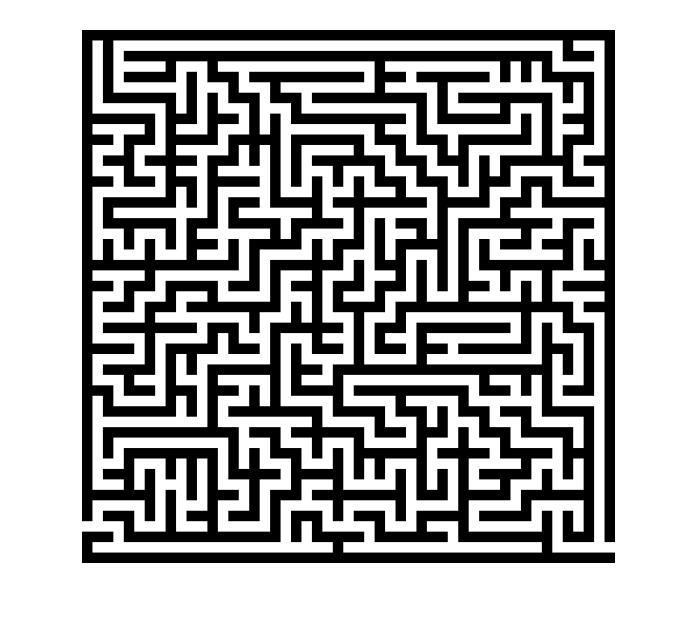

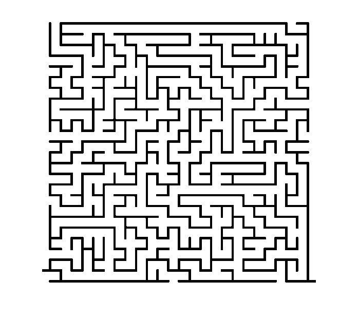
Make an image of walls by thresholding the maze image. Dilate the walls (make them a little thicker) in order to keep the solution path a little bit away from them.

walls = imdilate(I < 128, ones(7,7));
imshow(walls)

The function bwgeodesic will take seed locations (as column and row coordinates) in addition to binary images. Below I specify the seed locations as the two entry points into the maze.

D1 = bwdistgeodesic(~walls, 1, 497, 'quasi-euclidean');
D2 = bwdistgeodesic(~walls, 533, 517, 'quasi-euclidean');

The rest of the procedure is the same as above.

D = D1 + D2;
D = round(D * 8) / 8;

D(isnan(D)) = inf;
paths = imregionalmin(D);

solution_path = bwmorph(paths, 'thin', inf);
thick_solution_path = imdilate(solution_path, ones(3,3));
P = imoverlay(I, thick_solution_path, [1 0 0]);
imshow(P, 'InitialMagnification', 'fit')

(If you're interested in other maze-solving techniques using image processing, take a look at the File Exchange contribution maze_solution by Image Analyst.)

In a comment on part 1 of this series, Sepideh asked this question:

"I have a binary image which contains one pixel width skeleton of an image. I have got the skeleton using the bwmorph function. As you may know basically in this binary image, I have ones on the skeleton and zeros anywhere else. how can I find the shortest ‘quasi-euclidean’ distance between two nonzero elements which are on the skeleton? The path should be on the skeleton itself too."

The techniques described above can be applied to this path-along-a-skeleton problem. Let's try an example.

bw = imread('circles.png');
imshow(bw, 'InitialMagnification', 200)

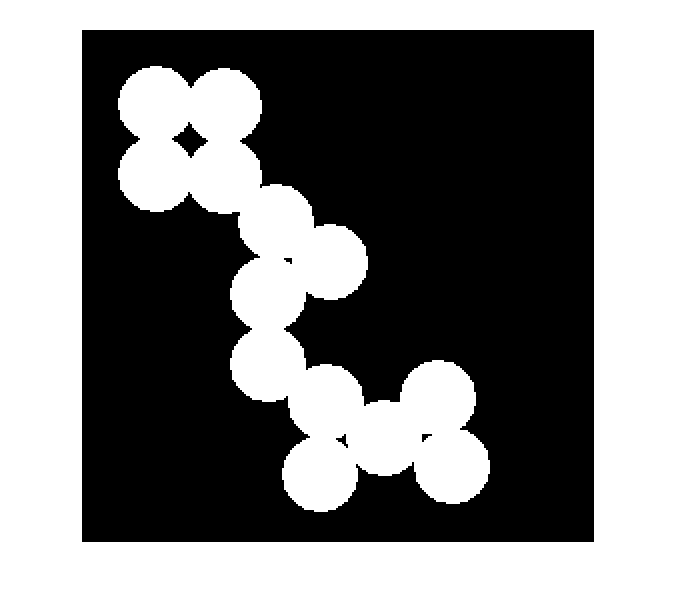
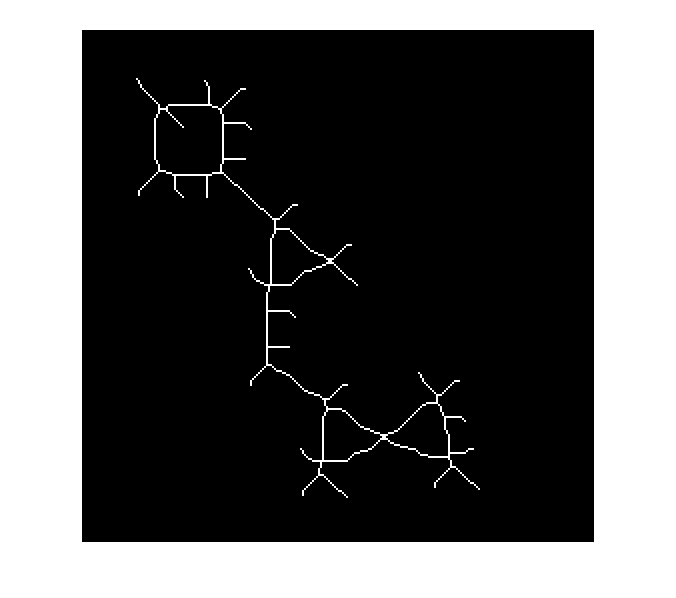
skel = bwmorph(bw, 'skel', Inf);
imshow(skel, 'InitialMagnification', 200)

Let's find the skeleton-constrained path distance between these two points.

r1 = 38;
c1 = 53;

r2 = 208;
c2 = 147;

hold on
plot(c1, r1, 'g*', 'MarkerSize', 15)
plot(c2, r2, 'g*', 'MarkerSize', 15)
hold off

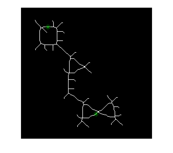
D1 = bwdistgeodesic(skel, c1, r1, 'quasi-euclidean');
D2 = bwdistgeodesic(skel, c2, r2, 'quasi-euclidean');

D = D1 + D2;
D = round(D * 8) / 8;

D(isnan(D)) = inf;
skeleton_path = imregionalmin(D);
P = imoverlay(skel, imdilate(skeleton_path, ones(3,3)), [1 0 0]);
imshow(P, 'InitialMagnification', 200)
hold on
plot(c1, r1, 'g*', 'MarkerSize', 15)
plot(c2, r2, 'g*', 'MarkerSize', 15)
hold off

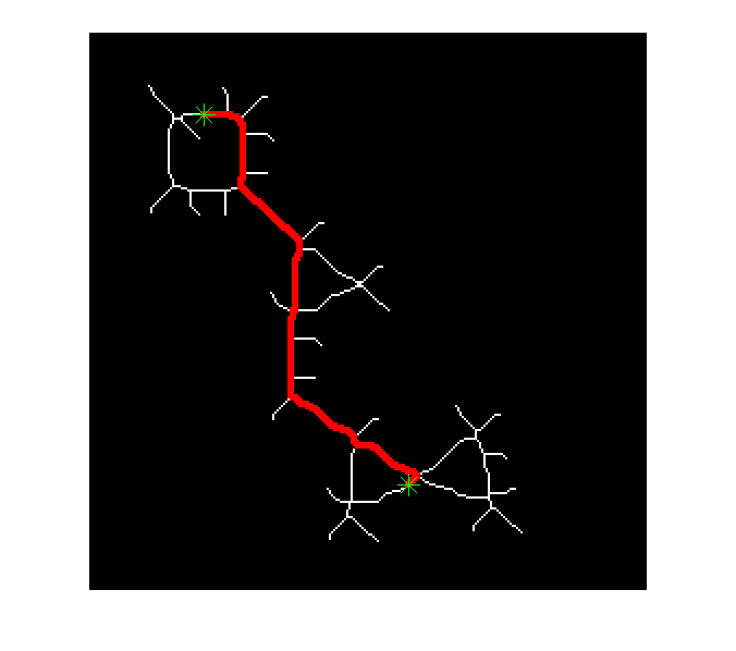
Finally, the skeleton path length is given by the value of D at any point along the path.

path_length = D(skeleton_path);
path_length = path_length(1)

path_length =

  239.2500

All the posts in this series

• the basic idea of finding shortest paths by adding two distance transforms together (part 1)
• the nonuniqueness of the shortest paths (part 2)
• handling floating-point round-off effects (part 3)
• using thinning to pick out a single path (part 4)
• using bwdistgeodesic to find shortest paths subject to constraint (part 5)

Get the MATLAB code

Published with MATLAB® 7.13